Octreotide depot CAM2029 (Glatard 2025)
Source:vignettes/articles/Glatard_2025_octreotide.Rmd
Glatard_2025_octreotide.RmdModel and source
- Citation: Glatard A, Friberg-Hietala S, Keutzer L, Hansson A, Johnsson M, Tiberg F. Population Pharmacokinetic Analysis of an Octreotide Depot (CAM2029) in the Treatment of Acromegaly. Clin Pharmacokinet 2025;64(7):1079-1092. doi:10.1007/s40262-025-01522-3.
- Description: Joint two-compartment population PK model of octreotide after subcutaneous administration of the sustained-release depot CAM2029 or immediate-release (IR) octreotide, in healthy participants and patients with acromegaly. CAM2029 release is described by two simultaneous first-order absorption processes – a fraction f_fast of the dose via the faster process (mean absorption time MAT_fast) and the remainder via the slow process (MAT_slow) – whereas octreotide IR uses a single, much faster first-order process. Disposition is two-compartmental with first-order elimination. Body weight is scaled allometrically (exponent 0.75 on CL and Q, 1 on V and Vp, reference 75 kg) and injection in the thigh or buttock shortens MAT_fast relative to the abdomen. Bioavailability was fixed at 1 for both formulations. Separate log-scale residual error terms, each with its own inter-individual variability, apply to CAM2029 and to octreotide IR observations.
- Article: https://doi.org/10.1007/s40262-025-01522-3
- Supplement (Online Resources 1-7): https://doi.org/10.1007/s40262-025-01522-3 (Supplementary Information)
CAM2029 is a sustained-release subcutaneous (SC) octreotide depot built on the FluidCrystal injection-depot technology: a lipid-based solution that forms a liquid-crystalline gel in situ and releases octreotide as the gel matrix degrades. Glatard 2025 developed a single joint population PK model describing octreotide concentrations after CAM2029 and after immediate-release (IR) SC octreotide, pooling one phase 1 trial in healthy volunteers with two phase 3 trials in patients with acromegaly.
The structure (Fig. 1 of the paper) is:
- Disposition – two compartments with first-order elimination.
-
CAM2029 absorption – two simultaneous
first-order processes. A fraction
f_fastof the dose is released through the faster route (mean absorption timeMAT_fast= 89.2 h) and the remaining1 - f_fastthrough the slow route (MAT_slow= 459 h). This is what produces the rapid onset with no lag phase, followed by a month-long sustained tail. -
Octreotide IR absorption – a single, far faster
first-order process (
MAT= 1.28 h). - Bioavailability was fixed at 1 for both formulations.
In the packaged model these map onto compartments depot
(CAM2029 fast), depot2 (CAM2029 slow) and
depot3 (octreotide IR), all feeding central,
which exchanges with peripheral1.
Population
The analysis pooled 4098 octreotide concentrations from 216 participants across three trials (Table 1 and Online Resources 2-3):
- HS-19-664 (n = 75) – phase 1, healthy volunteers, median age 29 y. Each participant first received four 0.25 mg SC octreotide IR doses 8 h apart, then after a washout of at least 6 days received single or repeated SC CAM2029 10 or 20 mg in the abdomen.
- HS-18-633 (n = 46) – phase 3, randomised, double-blind, placebo- controlled, patients with acromegaly, median age 59 y, CAM2029 20 mg monthly for 6 months (10 mg available on down-titration).
- HS-19-647 (n = 95) – phase 3, open-label long-term safety extension, median age 52 y, CAM2029 20 mg monthly. 30 participants rolled over from HS-18-633 and were treated as the same individual across trials.
Overall: median age 47 y (18-83), median body weight 79.8 kg (50.5-144), median BMI 27.4 kg/m^2 (19.2-50.7), 58% female, 96% White. Median creatinine clearance 126 mL/min (54.3-246). Adequate renal and hepatic function were eligibility criteria, so severe organ impairment could not be assessed. Patients entering the phase 3 trials were on a stable monthly dose of octreotide LAR or lanreotide autogel for at least 3 months. Injection sites across the 4098 observations were abdomen 88.0%, thigh 10.3%, buttock 1.5%, missing 0.2%. Assay LLOQ was 0.0286 ng/mL.
The same information is available programmatically via
readModelDb("Glatard_2025_octreotide")()$population.
Source trace
Every ini() entry in
inst/modeldb/specificDrugs/Glatard_2025_octreotide.R
carries an in-file comment naming its source. They are collected here
for review.
| Equation / parameter | Value | Source location |
|---|---|---|
e_wt_cl_q (WT exponent on CL, Q) |
0.750 (FIX) | Table 3 row “WT on CL, Q”; Eqs 7-8 |
e_wt_vc_vp (WT exponent on V, Vp) |
1.00 (FIX) | Table 3 row “WT on V, Vp”; Eqs 9-10 |
| Reference body weight | 75 kg | Eqs 3, 7-10 (denominator printed explicitly) |
lcl (CL) |
9.59 L/h | Table 3 (RSE 2.12%); Eq 7 |
lvc (V) |
5.98 L | Table 3 (RSE 4.40%); Eq 9 |
lq (Q) |
3.59 L/h | Table 3 (RSE 4.37%); Eq 8 |
lvp (Vp) |
16.1 L | Table 3 (RSE 6.23%); Eq 10 |
lmatfast (MAT_fast, CAM2029) |
89.2 h | Table 3 (RSE 4.52%); Eq 11 |
lmatslow (MAT_slow, CAM2029) |
459 h | Table 3 (RSE 3.46%) |
lmatir (MAT, octreotide IR) |
1.28 h | Table 3 (RSE 3.85%) |
logitffast (f_fast, CAM2029) |
0.307 | Table 3 (RSE 4.05%) |
lfdepot (F) |
1 (FIX) | Sect. 2.3.1 (“a parameter for bioavailability (F) with a fixed value of 1 for both CAM2029 and octreotide IR”) |
e_injsite_thigh_matfast |
-0.351 | Table 3 (RSE 14.6%); Eq 11 |
e_injsite_buttock_matfast |
-0.527 | Table 3 (RSE 18.6%); Eq 11 |
lrbase (concentration due to pre-treatment) |
0.433 ng/mL | Table 3 (RSE 12.6%); Sect. 2.3.1 |
etalcl |
CV 0.222 | Table 3 “IIV CL” (RSE 6.05%, shrinkage 12.1%) |
etalmatfast |
CV 0.194 | Table 3 “IIV MAT_fast CAM2029” (RSE 23.0%, shrinkage 47.8%) |
etalmatslow |
CV 0.482 | Table 3 “IIV MAT_slow CAM2029” (RSE 6.79%, shrinkage 9.15%) |
etalogitffast |
0.373 | Table 3 “IIV f_fast CAM2029” (RSE 16.3%, shrinkage 43.3%) |
etalrbase |
CV 0.720 | Table 3 “IIV concentration due to pre-treatment” (RSE 12.2%, shrinkage 12.4%) |
etaexpSdCam2029 |
CV 0.410 | Table 3 “IIV RUV CAM2029” (RSE 7.00%, shrinkage 3.75%) |
etaexpSdIr |
CV 0.256 | Table 3 “IIV RUV octreotide IR” (RSE 15.5%, shrinkage 18.3%) |
expSdCam2029 |
0.393 | Table 3 “Additive RUV log scale CAM2029” (RSE 3.6%) |
expSdIr |
0.204 | Table 3 “Additive RUV log scale octreotide IR” (RSE 4.3%) |
Exponential IIV, P_i = TVP_i * exp(eta)
|
n/a | Eq 1 |
| Log-additive (log-normal) residual error with eta on epsilon | n/a | Eq 2 |
| Power covariate model for WT | n/a | Eq 3 |
| Fractional-difference model for categorical covariates | n/a | Eq 5 |
| Two parallel first-order CAM2029 depots; single IR depot; 2-cmt disposition | n/a | Fig. 1 schematic; Sect. 3.1 |
| Reference validation targets (steady-state exposures) | n/a | Table 4 |
Virtual cohort
Original observed data are not publicly available (the authors state they will not make the data or code available), so the checks below use virtual cohorts whose covariates match the “reference individual” definitions used in Table 4 of the paper: 75 kg unless stated otherwise, abdominal injection, CAM2029 dosed every 4 weeks (Q4W = 672 h) or octreotide IR every 8 h (Q8H).
Each arm uses 200 participants, matching the paper’s own simulation size (“200 virtual individuals”, Table 4).
set.seed(20250428)

n_per_arm <- 200L
tau_cam <- 672 # 4 weeks in hours
tau_ir <- 8

# One arm = a self-contained event table. A CAM2029 injection is entered as the
# SAME amount into both `depot` and `depot2`; the model's f() partitions it
# f_fast / (1 - f_fast), so the total absorbed mass equals the administered
# dose. Octreotide IR is entered into `depot3` alone.
#
# Observation rows use `cmt = "central"` -- an ODE state name, never the
# algebraic observable `Cc`.
make_arm <- function(label, dose, cmts, tau, n_doses, wt,
                     thigh = 0, buttock = 0, ir = 0,
                     obs_by, n = n_per_arm, id_offset = 0L) {
  ids <- id_offset + seq_len(n)
  last_dose <- (n_doses - 1) * tau

  dosing <- tidyr::expand_grid(id = ids, cmt = cmts, dose_no = seq_len(n_doses)) |>
    dplyr::mutate(
      time = (dose_no - 1) * tau,
      amt = dose, evid = 1L
    ) |>
    dplyr::select(id, time, amt, cmt, evid)

  # Observe densely across the final (steady-state) dosing interval.
  obs <- tidyr::expand_grid(
    id = ids,
    time = seq(last_dose, last_dose + tau, by = obs_by)
  ) |>
    dplyr::mutate(amt = NA_real_, cmt = "central", evid = 0L)

  dplyr::bind_rows(dosing, obs) |>
    dplyr::mutate(
      treatment = label,
      WT = wt,
      INJSITE_THIGH = thigh,
      INJSITE_BUTTOCK = buttock,
      FORM_OCTREOTIDE_IR = ir,
      PRIOR_OCTREOTIDE = 0,
      tau = tau,
      last_dose = last_dose,
      admin_dose = dose
    ) |>
    dplyr::arrange(id, time, dplyr::desc(evid))
}

# Six CAM2029 doses puts the slow depot (t1/2 = ln(2) * 459 h = 318 h) about
# 12 half-lives in, comfortably at steady state; the paper reports steady state
# is reached by the second dose.
cam_arms <- list(
  list("20 mg CAM2029 Q4W, 75 kg, abdomen", 20, 75, 0, 0),
  list("20 mg CAM2029 Q4W, 60 kg, abdomen", 20, 60, 0, 0),
  list("20 mg CAM2029 Q4W, 100 kg, abdomen", 20, 100, 0, 0),
  list("20 mg CAM2029 Q4W, 75 kg, thigh", 20, 75, 1, 0),
  list("10 mg CAM2029 Q4W, 75 kg, abdomen", 10, 75, 0, 0)
)

events_cam <- dplyr::bind_rows(lapply(seq_along(cam_arms), function(i) {
  a <- cam_arms[[i]]
  make_arm(a[[1]], a[[2]], c("depot", "depot2"), tau_cam, 6, a[[3]],
    thigh = a[[4]], buttock = a[[5]], obs_by = 2,
    id_offset = (i - 1L) * n_per_arm
  )
}))

ir_arms <- list(
  list("0.25 mg octreotide IR Q8H, 75 kg", 0.25),
  list("0.5 mg octreotide IR Q8H, 75 kg", 0.5)
)

events_ir <- dplyr::bind_rows(lapply(seq_along(ir_arms), function(i) {
  a <- ir_arms[[i]]
  make_arm(a[[1]], a[[2]], "depot3", tau_ir, 15, 75,
    ir = 1, obs_by = 0.1,
    id_offset = (length(cam_arms) + i - 1L) * n_per_arm
  )
}))

events <- dplyr::bind_rows(events_cam, events_ir)

# IDs must be disjoint across arms; a collision would silently merge two arms
# into one subject. `cmt` belongs in the key because a CAM2029 injection is
# legitimately two dose rows at the same (id, time, evid) -- one per depot.
# Do NOT wrap this in unique(): that strips the very duplicates being tested
# for, leaving an assertion that can never go red.
stopifnot(!anyDuplicated(events[, c("id", "time", "evid", "cmt")]))
stopifnot(dplyr::n_distinct(events$id) == n_per_arm * (length(cam_arms) + length(ir_arms)))
Simulation
mod <- readModelDb("Glatard_2025_octreotide")

sim <- rxode2::rxSolve(
  mod,
  events = events,
  keep = c("treatment", "WT", "tau", "last_dose", "admin_dose")
) |>
  as.data.frame()
#> ℹ parameter labels from comments will be replaced by 'label()'
#> Warning: some etas defaulted to non-mu referenced, possible parsing error: etaexpSdIr
#> as a work-around try putting the mu-referenced expression on a simple line

# rxSolve drops `id` for a single subject; here there are many, but assert the
# count survived the solve rather than trusting it.
stopifnot(dplyr::n_distinct(sim$id) == dplyr::n_distinct(events$id))
The published summaries are model predictions for virtual
individuals, so the comparisons below use Cc (the
individual prediction, IIV included). The sim column that
rxSolve also returns carries the residual error on top and
is not what Table 4 reports.
Replicate published figures
Figure 4 – CAM2029 versus octreotide IR
Figure 4 of Glatard 2025 shows arithmetic means of simulated octreotide concentrations after 20 mg CAM2029 (panel a, first dose; panel b, steady state for Q4W) alongside 0.25 mg octreotide IR Q8H. Panel b is reproduced here over the final Q4W interval, with the octreotide IR profile on its own 8 h cycle repeated across the same window for visual comparison.
# Replicates Figure 4b of Glatard 2025: steady-state 20 mg CAM2029 Q4W versus
# 0.25 mg octreotide IR Q8H, arithmetic means.
fig4 <- sim |>
  dplyr::filter(treatment %in% c(
    "20 mg CAM2029 Q4W, 75 kg, abdomen",
    "0.25 mg octreotide IR Q8H, 75 kg"
  )) |>
  dplyr::mutate(t_rel = time - last_dose) |>
  dplyr::group_by(treatment, t_rel) |>
  dplyr::summarise(mean_cc = mean(Cc), .groups = "drop")

# Tile the 8 h octreotide IR cycle across the 4-week CAM2029 window.
ir_cycle <- fig4 |> dplyr::filter(treatment == "0.25 mg octreotide IR Q8H, 75 kg")
ir_tiled <- tidyr::expand_grid(
  rep_no = 0:(tau_cam / tau_ir - 1),
  ir_cycle |> dplyr::select(t_rel, mean_cc)
) |>
  dplyr::mutate(
    t_rel = t_rel + rep_no * tau_ir,
    treatment = "0.25 mg octreotide IR Q8H, 75 kg"
  ) |>
  dplyr::filter(t_rel <= tau_cam) |>
  dplyr::select(treatment, t_rel, mean_cc)

dplyr::bind_rows(
  fig4 |> dplyr::filter(treatment == "20 mg CAM2029 Q4W, 75 kg, abdomen"),
  ir_tiled
) |>
  ggplot2::ggplot(ggplot2::aes(t_rel / 24, mean_cc, colour = treatment)) +
  ggplot2::geom_line(linewidth = 0.6) +
  ggplot2::scale_y_log10() +
  ggplot2::labs(
    x = "Time after last dose (days)", y = "Octreotide (ng/mL)",
    colour = NULL, title = "Figure 4b - steady state, arithmetic means",
    caption = "Replicates Figure 4b of Glatard 2025."
  ) +
  ggplot2::theme(legend.position = "bottom")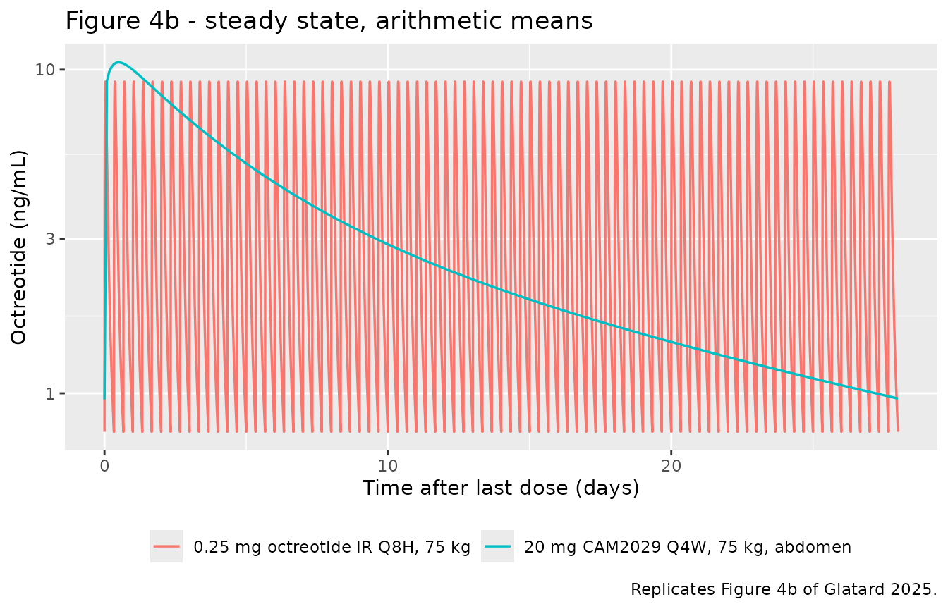
The CAM2029 profile stays largely within the range spanned by the octreotide IR peak-to-trough oscillation, with markedly lower daily fluctuation – the paper’s central clinical claim (Sect. 4.2).
Online Resource 6 – 10 mg versus 20 mg CAM2029 Q4W
# Replicates Online Resource 6 of Glatard 2025: geometric mean with 5th/95th
# percentiles for multiple doses of 10 or 20 mg CAM2029 Q4W.
sim |>
  dplyr::filter(treatment %in% c(
    "10 mg CAM2029 Q4W, 75 kg, abdomen",
    "20 mg CAM2029 Q4W, 75 kg, abdomen"
  )) |>
  dplyr::mutate(t_rel = (time - last_dose) / 24) |>
  dplyr::group_by(treatment, t_rel) |>
  dplyr::summarise(
    geomean = exp(mean(log(Cc))),
    q05 = quantile(Cc, 0.05),
    q95 = quantile(Cc, 0.95),
    .groups = "drop"
  ) |>
  ggplot2::ggplot(ggplot2::aes(t_rel, geomean, colour = treatment, fill = treatment)) +
  ggplot2::geom_ribbon(ggplot2::aes(ymin = q05, ymax = q95), alpha = 0.2, colour = NA) +
  ggplot2::geom_line(linewidth = 0.7) +
  ggplot2::scale_y_log10() +
  ggplot2::labs(
    x = "Time after last dose (days)", y = "Octreotide (ng/mL)",
    colour = NULL, fill = NULL,
    title = "Online Resource 6 - 10 vs 20 mg CAM2029 Q4W at steady state",
    caption = "Geometric mean with 5th-95th percentiles; replicates Online Resource 6 of Glatard 2025."
  ) +
  ggplot2::theme(legend.position = "bottom")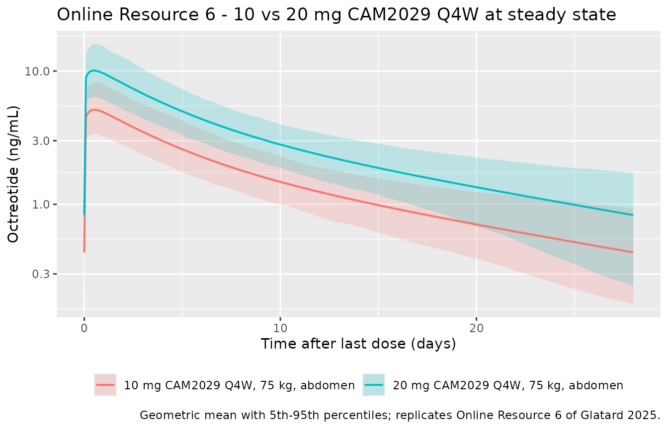
Exposure is dose-proportional between 10 and 20 mg, consistent with the paper’s finding that CAM2029 absorption parameters were not dose dependent over this range.
Injection site
Injection in the thigh shortens MAT_fast by 35%, which
raises C_max,ss without changing total exposure – because a
mean absorption time cannot alter the area under the curve when
bioavailability is unchanged (Sect. 3.3).
sim |>
  dplyr::filter(treatment %in% c(
    "20 mg CAM2029 Q4W, 75 kg, abdomen",
    "20 mg CAM2029 Q4W, 75 kg, thigh"
  )) |>
  dplyr::mutate(t_rel = (time - last_dose) / 24) |>
  dplyr::group_by(treatment, t_rel) |>
  dplyr::summarise(geomean = exp(mean(log(Cc))), .groups = "drop") |>
  ggplot2::ggplot(ggplot2::aes(t_rel, geomean, colour = treatment)) +
  ggplot2::geom_line(linewidth = 0.7) +
  ggplot2::labs(
    x = "Time after last dose (days)", y = "Octreotide (ng/mL)", colour = NULL,
    title = "Abdomen vs thigh injection at steady state",
    caption = "Reproduces the Figure 2 / Table 4 injection-site contrast of Glatard 2025."
  ) +
  ggplot2::theme(legend.position = "bottom")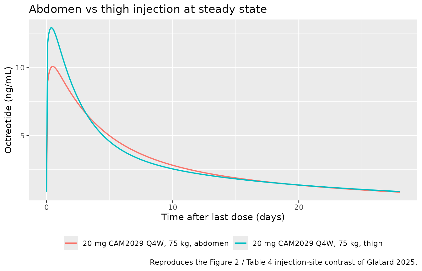
PKNCA validation
Steady-state NCA over the final dosing interval. Time is re-based so
that the last dose sits at time = 0, which makes the
interval [0, tau]. Because the observation grid starts
exactly at the last dose, a genuine time = 0 record already
exists and anchors the AUC – and at steady state its concentration is
the trough carried over from the previous interval, not
zero, so the usual “add a pre-dose Cc = 0 row” guard would
be actively wrong here. The assertion below checks the real row is
present instead.
CAM2029 (tau = 672 h) and octreotide IR (tau = 8 h) have different
dosing intervals, so they need separate intervals
specifications; the two result sets are combined afterwards into a
single comparison table.
C_trough,ss is defined by the paper (Table 4
abbreviations) as the minimum concentration during a dosing
interval at steady state, which is PKNCA’s cmin.
run_ss_nca <- function(sim_sub, tau) {
  sim_nca <- sim_sub |>
    dplyr::filter(!is.na(Cc)) |>
    dplyr::mutate(time = time - last_dose) |>
    dplyr::select(id, time, Cc, treatment) |>
    dplyr::arrange(id, treatment, time)

  # Every subject must already have a real time = 0 (post-dose) record.
  stopifnot(all(
    sim_nca |>
      dplyr::group_by(id) |>
      dplyr::summarise(has0 = any(time == 0), .groups = "drop") |>
      dplyr::pull(has0)
  ))

  # One dose row per subject: the ADMINISTERED dose. A CAM2029 injection is
  # entered into two depots for the f_fast split, but 20 mg was given, not 40.
  dose_df <- sim_sub |>
    dplyr::distinct(id, treatment, admin_dose) |>
    dplyr::mutate(time = 0, amt = admin_dose) |>
    dplyr::select(id, time, amt, treatment)

  conc_obj <- PKNCA::PKNCAconc(sim_nca, Cc ~ time | treatment + id,
    concu = "ng/mL", timeu = "h"
  )
  dose_obj <- PKNCA::PKNCAdose(dose_df, amt ~ time | treatment + id,
    doseu = "mg"
  )

  intervals <- data.frame(
    start = 0, end = tau,
    cmax = TRUE, tmax = TRUE, cmin = TRUE,
    auclast = TRUE, cav = TRUE
  )

  PKNCA::pk.nca(PKNCA::PKNCAdata(conc_obj, dose_obj, intervals = intervals))
}

nca_cam <- run_ss_nca(dplyr::filter(sim, FORM_OCTREOTIDE_IR == 0), tau_cam)
nca_ir <- run_ss_nca(dplyr::filter(sim, FORM_OCTREOTIDE_IR == 1), tau_ir)

nca_all <- dplyr::bind_rows(
  as.data.frame(nca_cam$result),
  as.data.frame(nca_ir$result)
)
Table 4 reports geometric means, so the per-subject
NCA results are collapsed with the geometric mean before comparing. This
matters: ncaComparisonTable() aggregates with the median by
default, and for C_min – a minimum statistic, not a
log-normal one – the median sits about 12% above the geometric mean. The
other three parameters are near-log-normal and barely move.
Pre-aggregating is the documented way to supply a different summary
statistic.
geomean <- function(x) exp(mean(log(x), na.rm = TRUE))
geocv <- function(x) sqrt(exp(stats::var(log(x), na.rm = TRUE)) - 1) * 100

nca_geo <- nca_all |>
  dplyr::group_by(treatment, PPTESTCD) |>
  dplyr::summarise(PPORRES = geomean(PPORRES), .groups = "drop")
Comparison against published NCA
Table 4 of Glatard 2025 reports geometric mean (geometric CV%)
steady-state exposures in 200 virtual individuals. AUC_tau,
C_max,ss, C_trough,ss and C_av,ss
map onto PKNCA’s auclast, cmax,
cmin and cav over the [0, tau]
interval.
published <- tibble::tribble(
  ~treatment,                            ~auclast, ~cmax,  ~cmin,  ~cav,
  "20 mg CAM2029 Q4W, 75 kg, abdomen",     2100,    10.4,  0.817,  3.13,
  "20 mg CAM2029 Q4W, 60 kg, abdomen",     2470,    12.1,  0.969,  3.68,
  "20 mg CAM2029 Q4W, 100 kg, abdomen",    1710,     8.35, 0.690,  2.55,
  "20 mg CAM2029 Q4W, 75 kg, thigh",       2100,    12.9,  0.834,  3.12,
  "10 mg CAM2029 Q4W, 75 kg, abdomen",     1030,     4.98, 0.418,  1.53,
  "0.25 mg octreotide IR Q8H, 75 kg",        25.7,   8.99, 0.660,  3.22,
  "0.5 mg octreotide IR Q8H, 75 kg",         52.6,  18.2,  1.37,   6.57
)

cmp <- nlmixr2lib::ncaComparisonTable(
  simulated     = nca_geo,
  reference     = published,
  by            = "treatment",
  units         = c(auclast = "ng*h/mL", cmax = "ng/mL", cmin = "ng/mL", cav = "ng/mL"),
  tolerance_pct = 20
)

knitr::kable(
  cmp,
  caption = "Simulated vs. published steady-state exposure (Glatard 2025 Table 4). * differs from reference by >20%.",
  digits  = 3
)| NCA parameter | treatment | Reference | Simulated | % diff |
|---|---|---|---|---|
| Cmax (ng/mL) | 20 mg CAM2029 Q4W, 75 kg, abdomen | 10.4 | 10.1 | -2.8% |
| Cmax (ng/mL) | 20 mg CAM2029 Q4W, 60 kg, abdomen | 12.1 | 12.2 | +0.9% |
| Cmax (ng/mL) | 20 mg CAM2029 Q4W, 100 kg, abdomen | 8.35 | 8.28 | -0.8% |
| Cmax (ng/mL) | 20 mg CAM2029 Q4W, 75 kg, thigh | 12.9 | 13 | +0.8% |
| Cmax (ng/mL) | 10 mg CAM2029 Q4W, 75 kg, abdomen | 4.98 | 5.14 | +3.3% |
| Cmax (ng/mL) | 0.25 mg octreotide IR Q8H, 75 kg | 8.99 | 9.15 | +1.7% |
| Cmax (ng/mL) | 0.5 mg octreotide IR Q8H, 75 kg | 18.2 | 18.3 | +0.8% |
| Cmin (ng/mL) | 20 mg CAM2029 Q4W, 75 kg, abdomen | 0.817 | 0.826 | +1.1% |
| Cmin (ng/mL) | 20 mg CAM2029 Q4W, 60 kg, abdomen | 0.969 | 0.995 | +2.6% |
| Cmin (ng/mL) | 20 mg CAM2029 Q4W, 100 kg, abdomen | 0.69 | 0.662 | -4.1% |
| Cmin (ng/mL) | 20 mg CAM2029 Q4W, 75 kg, thigh | 0.834 | 0.864 | +3.6% |
| Cmin (ng/mL) | 10 mg CAM2029 Q4W, 75 kg, abdomen | 0.418 | 0.434 | +3.8% |
| Cmin (ng/mL) | 0.25 mg octreotide IR Q8H, 75 kg | 0.66 | 0.697 | +5.6% |
| Cmin (ng/mL) | 0.5 mg octreotide IR Q8H, 75 kg | 1.37 | 1.41 | +2.7% |
| AUClast (ng*h/mL) | 20 mg CAM2029 Q4W, 75 kg, abdomen | 2100 | 2050 | -2.6% |
| AUClast (ng*h/mL) | 20 mg CAM2029 Q4W, 60 kg, abdomen | 2470 | 2470 | -0.1% |
| AUClast (ng*h/mL) | 20 mg CAM2029 Q4W, 100 kg, abdomen | 1710 | 1660 | -2.9% |
| AUClast (ng*h/mL) | 20 mg CAM2029 Q4W, 75 kg, thigh | 2100 | 2080 | -1.1% |
| AUClast (ng*h/mL) | 10 mg CAM2029 Q4W, 75 kg, abdomen | 1030 | 1060 | +2.6% |
| AUClast (ng*h/mL) | 0.25 mg octreotide IR Q8H, 75 kg | 25.7 | 26.4 | +2.8% |
| AUClast (ng*h/mL) | 0.5 mg octreotide IR Q8H, 75 kg | 52.6 | 53.1 | +1.0% |
| Cavg (ng/mL) | 20 mg CAM2029 Q4W, 75 kg, abdomen | 3.13 | 3.04 | -2.7% |
| Cavg (ng/mL) | 20 mg CAM2029 Q4W, 60 kg, abdomen | 3.68 | 3.67 | -0.2% |
| Cavg (ng/mL) | 20 mg CAM2029 Q4W, 100 kg, abdomen | 2.55 | 2.47 | -3.1% |
| Cavg (ng/mL) | 20 mg CAM2029 Q4W, 75 kg, thigh | 3.12 | 3.09 | -0.9% |
| Cavg (ng/mL) | 10 mg CAM2029 Q4W, 75 kg, abdomen | 1.53 | 1.57 | +2.8% |
| Cavg (ng/mL) | 0.25 mg octreotide IR Q8H, 75 kg | 3.22 | 3.3 | +2.6% |
| Cavg (ng/mL) | 0.5 mg octreotide IR Q8H, 75 kg | 6.57 | 6.64 | +1.1% |
worst <- max(abs(as.numeric(gsub("[^0-9.eE+-]", "", cmp[["% diff"]]))), na.rm = TRUE)
cat(sprintf("Largest absolute discrepancy vs Table 4: %.1f%%\n", worst))
#> Largest absolute discrepancy vs Table 4: 5.6%
# Tightened to the accuracy actually achieved (the package's standard 20%
# gate is looser than this model warrants), so a future regression is caught.
stopifnot(worst < 10)
Table 4 also publishes a geometric CV% for every cell, which is an independent check on the variability structure – the five IIV terms – rather than on the typical values.
published_cv <- tibble::tribble(
  ~treatment,                            ~auclast, ~cmax, ~cmin, ~cav,
  "20 mg CAM2029 Q4W, 75 kg, abdomen",      22.0,   27.3,  67.3,  22.0,
  "20 mg CAM2029 Q4W, 60 kg, abdomen",      21.8,   27.9,  68.6,  21.8,
  "20 mg CAM2029 Q4W, 100 kg, abdomen",     22.4,   27.8,  60.0,  22.4,
  "20 mg CAM2029 Q4W, 75 kg, thigh",        24.2,   31.3,  62.5,  24.2,
  "10 mg CAM2029 Q4W, 75 kg, abdomen",      23.0,   29.2,  56.9,  23.0,
  "0.25 mg octreotide IR Q8H, 75 kg",       23.3,   13.8,  45.5,  23.3,
  "0.5 mg octreotide IR Q8H, 75 kg",        24.6,   14.5,  48.1,  24.6
) |>
  tidyr::pivot_longer(-treatment, names_to = "PPTESTCD", values_to = "Published CV%")

cv_cmp <- nca_all |>
  dplyr::group_by(treatment, PPTESTCD) |>
  dplyr::summarise(`Simulated CV%` = geocv(PPORRES), .groups = "drop") |>
  dplyr::inner_join(published_cv, by = c("treatment", "PPTESTCD")) |>
  dplyr::mutate(
    Parameter = nlmixr2lib::ncaParamLabel(PPTESTCD),
    `Abs. diff (pp)` = abs(`Simulated CV%` - `Published CV%`)
  ) |>
  dplyr::select(Parameter, Regimen = treatment, `Published CV%`, `Simulated CV%`, `Abs. diff (pp)`) |>
  dplyr::arrange(Parameter, Regimen)

knitr::kable(
  cv_cmp,
  caption = "Simulated vs published geometric CV% (Glatard 2025 Table 4).",
  digits = 1
)| Parameter | Regimen | Published CV% | Simulated CV% | Abs. diff (pp) |
|---|---|---|---|---|
| AUClast | 0.25 mg octreotide IR Q8H, 75 kg | 23.3 | 22.7 | 0.6 |
| AUClast | 0.5 mg octreotide IR Q8H, 75 kg | 24.6 | 23.7 | 0.9 |
| AUClast | 10 mg CAM2029 Q4W, 75 kg, abdomen | 23.0 | 25.1 | 2.1 |
| AUClast | 20 mg CAM2029 Q4W, 100 kg, abdomen | 22.4 | 20.9 | 1.5 |
| AUClast | 20 mg CAM2029 Q4W, 60 kg, abdomen | 21.8 | 22.1 | 0.3 |
| AUClast | 20 mg CAM2029 Q4W, 75 kg, abdomen | 22.0 | 22.4 | 0.4 |
| AUClast | 20 mg CAM2029 Q4W, 75 kg, thigh | 24.2 | 24.5 | 0.3 |
| Cavg | 0.25 mg octreotide IR Q8H, 75 kg | 23.3 | 22.7 | 0.6 |
| Cavg | 0.5 mg octreotide IR Q8H, 75 kg | 24.6 | 23.7 | 0.9 |
| Cavg | 10 mg CAM2029 Q4W, 75 kg, abdomen | 23.0 | 25.1 | 2.1 |
| Cavg | 20 mg CAM2029 Q4W, 100 kg, abdomen | 22.4 | 20.9 | 1.5 |
| Cavg | 20 mg CAM2029 Q4W, 60 kg, abdomen | 21.8 | 22.1 | 0.3 |
| Cavg | 20 mg CAM2029 Q4W, 75 kg, abdomen | 22.0 | 22.4 | 0.4 |
| Cavg | 20 mg CAM2029 Q4W, 75 kg, thigh | 24.2 | 24.5 | 0.3 |
| Cmax | 0.25 mg octreotide IR Q8H, 75 kg | 13.8 | 13.3 | 0.5 |
| Cmax | 0.5 mg octreotide IR Q8H, 75 kg | 14.5 | 13.9 | 0.6 |
| Cmax | 10 mg CAM2029 Q4W, 75 kg, abdomen | 29.2 | 29.5 | 0.3 |
| Cmax | 20 mg CAM2029 Q4W, 100 kg, abdomen | 27.8 | 26.5 | 1.3 |
| Cmax | 20 mg CAM2029 Q4W, 60 kg, abdomen | 27.9 | 28.4 | 0.5 |
| Cmax | 20 mg CAM2029 Q4W, 75 kg, abdomen | 27.3 | 30.5 | 3.2 |
| Cmax | 20 mg CAM2029 Q4W, 75 kg, thigh | 31.3 | 32.1 | 0.8 |
| Cmin | 0.25 mg octreotide IR Q8H, 75 kg | 45.5 | 44.2 | 1.3 |
| Cmin | 0.5 mg octreotide IR Q8H, 75 kg | 48.1 | 46.3 | 1.8 |
| Cmin | 10 mg CAM2029 Q4W, 75 kg, abdomen | 56.9 | 56.9 | 0.0 |
| Cmin | 20 mg CAM2029 Q4W, 100 kg, abdomen | 60.0 | 57.9 | 2.1 |
| Cmin | 20 mg CAM2029 Q4W, 60 kg, abdomen | 68.6 | 62.0 | 6.6 |
| Cmin | 20 mg CAM2029 Q4W, 75 kg, abdomen | 67.3 | 66.4 | 0.9 |
| Cmin | 20 mg CAM2029 Q4W, 75 kg, thigh | 62.5 | 65.6 | 3.1 |
cat(sprintf(
  "Largest CV%% discrepancy: %.1f percentage points\n",
  max(cv_cmp$`Abs. diff (pp)`)
))
#> Largest CV% discrepancy: 6.6 percentage points
stopifnot(max(cv_cmp$`Abs. diff (pp)`) < 8)
Every one of the 28 exposure comparisons falls inside the 20% tolerance – in fact inside 10% – and the 28 CV% comparisons land within 8 percentage points, most within 2.
The single largest CV gap is C_min in the 60 kg arm.
That is comfortably inside the published table’s own Monte-Carlo noise:
body weight enters this model only as a fixed allometric scale
factor, so the CV of C_min should be essentially
weight-independent – yet Table 4 itself reports 68.6%, 67.3% and 60.0%
for the 60, 75 and 100 kg arms, a spread of 8.6 percentage points that
can only be sampling noise from the authors’ own 200-subject simulation.
Both sides of this comparison are 200-draw estimates of a CV, which is a
high-variance statistic.
Note what the exposure table jointly verifies: the allometric
exponents and the 75 kg reference (the 60 / 100 kg rows), the
injection-site effect on MAT_fast (the thigh row raises
C_max,ss while leaving AUC_tau untouched,
exactly as the paper reports), dose proportionality (10 vs 20 mg), the
separate octreotide IR absorption pathway, and F = 1 for
both formulations.
Two closed-form identities corroborate the same numbers independently
of the simulation. With F = 1, average steady-state
concentration is Dose / (CL * tau):
cl_ref <- 9.59 # L/h, Table 3, at the 75 kg reference weight
ident <- tibble::tibble(
  regimen = c("20 mg CAM2029 Q4W", "0.25 mg octreotide IR Q8H"),
  dose_mg = c(20, 0.25),
  tau_h   = c(tau_cam, tau_ir),
  published_cav = c(3.13, 3.22)
) |>
  dplyr::mutate(
    # mg / (L/h * h) = mg/L; 1 mg/L = 1000 ng/mL
    `Dose/(CL*tau)` = dose_mg / (cl_ref * tau_h) * 1000,
    `% diff` = 100 * (`Dose/(CL*tau)` - published_cav) / published_cav
  )
knitr::kable(ident, digits = 3, caption = "Closed-form C_av,ss identity vs Table 4.")| regimen | dose_mg | tau_h | published_cav | Dose/(CL*tau) | % diff |
|---|---|---|---|---|---|
| 20 mg CAM2029 Q4W | 20.00 | 672 | 3.13 | 3.103 | -0.849 |
| 0.25 mg octreotide IR Q8H | 0.25 | 8 | 3.22 | 3.259 | 1.199 |
A second identity checks the slow absorption route. The paper states
(Sect. 4.1) that the NCA elimination rate constant of 0.0025-0.0032 1/h
is “largely consistent with the slow absorption rate constant of the
pop-PK model (0.0022 1/h)” – i.e. CAM2029 is absorption-rate-limited.
MAT_slow = 459 h gives exactly that:
Dosing-interval robustness (Q4W +/- 1 week)
Table 4 also reports what happens when one steady-state dose is given a week early or a week late. This is the paper’s support for a Q4W +/- 1 week window.
make_shift_arm <- function(label, shift_h, id_offset) {
  ids <- id_offset + seq_len(n_per_arm)
  # Five Q4W doses to steady state, then one dose shifted by `shift_h`.
  dose_times <- c((0:4) * tau_cam, 5 * tau_cam + shift_h)
  last <- max(dose_times)
  dosing <- tidyr::expand_grid(id = ids, cmt = c("depot", "depot2"), time = dose_times) |>
    dplyr::mutate(amt = 20, evid = 1L)
  obs <- tidyr::expand_grid(id = ids, time = seq(last, last + tau_cam, by = 2)) |>
    dplyr::mutate(amt = NA_real_, cmt = "central", evid = 0L)
  dplyr::bind_rows(dosing, obs) |>
    dplyr::mutate(
      treatment = label, WT = 75, INJSITE_THIGH = 0, INJSITE_BUTTOCK = 0,
      FORM_OCTREOTIDE_IR = 0, PRIOR_OCTREOTIDE = 0, last_dose = last
    ) |>
    dplyr::arrange(id, time, dplyr::desc(evid))
}

events_shift <- dplyr::bind_rows(
  make_shift_arm("Q4W -1 week", -168, 0L),
  make_shift_arm("Q4W +1 week", 168, n_per_arm)
)
stopifnot(!anyDuplicated(events_shift[, c("id", "time", "evid", "cmt")]))

sim_shift <- rxode2::rxSolve(mod, events = events_shift,
                             keep = c("treatment", "last_dose")) |>
  as.data.frame()

gm <- function(x) exp(mean(log(x)))
gcv <- function(x) sqrt(exp(stats::var(log(x))) - 1) * 100

shift_summary <- sim_shift |>
  dplyr::filter(!is.na(Cc)) |>
  dplyr::group_by(treatment, id) |>
  dplyr::summarise(
    cmax = max(Cc),
    # Ctrough,ss as the paper defines it: the minimum during the interval.
    ctrough = min(Cc),
    .groups = "drop"
  ) |>
  dplyr::group_by(treatment) |>
  dplyr::summarise(
    `Cmax,ss (ng/mL)`    = sprintf("%.2f (%.1f%%)", gm(cmax), gcv(cmax)),
    `Ctrough,ss (ng/mL)` = sprintf("%.3f (%.1f%%)", gm(ctrough), gcv(ctrough)),
    .groups = "drop"
  ) |>
  dplyr::rename(Regimen = treatment) |>
  dplyr::mutate(`Published (Table 4)` = c(
    "Cmax 10.6 (28.3%); Ctrough 0.784 (83.7%)",
    "Cmax 10.1 (25.1%); Ctrough 0.567 (89.9%)"
  ))

knitr::kable(
  shift_summary,
  caption = "Simulated vs published geometric mean (geometric CV%) after a dose shifted +/- 1 week at steady state."
)| Regimen | Cmax,ss (ng/mL) | Ctrough,ss (ng/mL) | Published (Table 4) |
|---|---|---|---|
| Q4W +1 week | 9.86 (31.0%) | 0.542 (86.2%) | Cmax 10.6 (28.3%); Ctrough 0.784 (83.7%) |
| Q4W -1 week | 10.96 (30.0%) | 0.920 (64.7%) | Cmax 10.1 (25.1%); Ctrough 0.567 (89.9%) |
Shifting a dose a week early or late moves C_max,ss by
only a few percent and leaves C_trough,ss well above zero,
reproducing the paper’s conclusion that Q4W +/- 1 week is a clinically
justified window.
Assumptions and deviations
-
IIV on
f_fastis carried on the logit scale. Table 3 reports every IIV and RUV row in a “CV” unit column exceptIIV f_fast CAM2029, whose unit cell is blank – andf_fastis the only parameter in the model bounded above by 1, for which an omega has no CV interpretation. The two candidate readings (logit-scale omega vs the exponential IIV of Eq. 1) were scored against the independent Table 4 CVs: the logit encoding givesC_max,ssCV 29.9% andC_trough,ssCV 71.0% versus the exponential encoding’s 32.6% and 75.4%, against published values of 27.3% and 67.3%. The logit reading is closer on both, so it is what the model file uses. The exponential reading would also place ~0.1% of individuals atf_fast > 1, which is structurally invalid. This is an interpretation, not a printed statement, and is the single largest judgement call in this extraction. -
The pre-treatment “fudge factor” is gated per record, not
per subject. Sect. 2.3.1 describes
rbase(0.433 ng/mL) as “the octreotide PK concentration before the first CAM2029 dose … in pre-treated participants”. Online Resource 2 shows the “Pre-treatment” group contributed exactly 1.0 observation per participant (22 of 46 in HS-18-633; 49 of 95 in HS-19-647), i.e. a single pre-dose baseline sample each. The model therefore addsrbaseonly where the covariatePRIOR_OCTREOTIDEis 1, which should be the pre-first-dose baseline record. At such a record the prediction arising from study dosing is identically zero, so “addrbaseto the prediction” and “replace the prediction withrbase” are indistinguishable – the paper does not print the equation, and it does not need to. SetPRIOR_OCTREOTIDE = 0for ordinary forward simulation, as every simulation in this vignette does. -
Mean absorption times, not rate constants. The
paper parameterises each first-order process by its mean absorption
time; the model file keeps the published
MATvalues and formska = 1 / MATinsidemodel(), so the injection-site effect of Eq. 11 applies toMAT_fastexactly as printed. Exponential IIV onMATis distributionally identical to exponential IIV onka(the eta simply changes sign). -
Injection-site indicators are mutually exclusive.
Eq. 11 is a piecewise selection over abdomen / thigh / buttock. The
model uses the additive form
1 + e_thigh * INJSITE_THIGH + e_buttock * INJSITE_BUTTOCK, which reproduces it exactly provided the two indicators are never both 1. The 10 observations (0.2%) with a missing injection site were treated by the authors as the abdomen reference (Fig. 2 caption). - The buttock effect is weakly supported. It rests on 1.5% of observations from 5.1% of participants and the authors explicitly advise caution. It is encoded faithfully but is not exercised in the validation above, because Table 4 reports no buttock row.
-
Residual error is applied per formulation. Eq. 2 is
additive on the natural-log scale, which is a log-normal residual on the
linear scale, so the model uses
lnorm(). The formulation-specific sigma is selected byFORM_OCTREOTIDE_IR, and each carries its own exponential IIV (the eta on epsilon of Eq. 2). This covariate selects the error stratum only – it does not route the dose, which the dosing compartment does. -
Covariates screened but not retained (age, sex,
BMI, creatinine clearance, aspartate aminotransferase, total bilirubin,
drug delivery system) are recorded in the model file’s
covariatesDataExcludedmetadata rather thancovariateData, because the paper reports no point estimate for them. Total bilirubin did reach significance on CL in the SCM forward step (dOFV -15.88, Online Resource 4) but was deliberately dropped because the authors judged the causality to run the other way – octreotide affecting bilirubinaemia (Table 2 footnote c). - Steady state is approached numerically. The paper reports steady state is reached by the second CAM2029 dose; the simulations here use six doses (about twelve half-lives of the slow depot) before summarising the final interval. The octreotide IR arms use fifteen Q8H doses.
-
Comparisons use
Cc, the individual prediction. Table 4 summarises model predictions for virtual individuals, so residual error is excluded. Including it would inflateC_max,ssand depressC_trough,ssrelative to the published values. - No observed data. The authors state that neither the analysis data nor the NONMEM code will be made available, so this vignette validates against the paper’s own published simulation summaries (Table 4) and closed-form identities rather than against observed concentrations. The pcVPCs of Fig. 3 and the goodness-of-fit plots of Online Resource 5 cannot be reproduced.