Nivolumab in Chinese patients (Zhang 2019)
Source:vignettes/articles/Zhang_2019b_nivolumab.Rmd
Zhang_2019b_nivolumab.RmdModel and source
- Citation: Zhang J, Cai J, Bello A, Roy A, Sheng J. Model-Based Population Pharmacokinetic Analysis of Nivolumab in Chinese Patients With Previously Treated Advanced Solid Tumors, Including Non-Small Cell Lung Cancer. J Clin Pharmacol. 2019;59(10):1415-1424. doi:[10.1002/jcph.1432](https://doi.org/10.1002/jcph.1432)
- Article: https://doi.org/10.1002/jcph.1432
- Supporting information (Tables S1-S7): https://europepmc.org/article/PMC/PMC6767401
- Description: Two-compartment population PK model with sigmoidal time-varying clearance for intravenous nivolumab (anti-PD-1 IgG4) in Chinese and global patients with previously treated advanced solid tumors, including NSCLC and nasopharyngeal carcinoma (Zhang 2019, J Clin Pharmacol)
- Modality: Therapeutic monoclonal antibody (IgG4), IV infusion.
Nivolumab is a fully human anti-PD-1 IgG4 monoclonal antibody. This
analysis re-estimated the parameters of the Bajaj 2017
global nivolumab monotherapy population-PK model (packaged here as
Bajaj_2017_nivolumab) on a pooled data set that added a
Chinese cohort, and revised the tumor-type covariate so that both NSCLC
(the reference) and nasopharyngeal carcinoma (NPC) carry explicit
levels. Its purpose was regulatory: to show that nivolumab PK is not
sensitive to race, and to bracket the exposure of a 240 mg flat-dose
regimen in Chinese patients against the approved 3 mg/kg Q2W
regimen.
Structure: linear two-compartment IV model with time-varying CL via a sigmoid-Emax function of time since the start of treatment,
and baseline clearance (Zhang 2019 p. 1418)
The exponential terms are printed in the source without their 0/1 indicators; each applies only to subjects in that category. The reference patient (Figure 1 caption) is a white/other male, 80 kg, ECOG PS 0, eGFR 90 mL/min/1.73 m^2, second-line-or-later NSCLC, and carries none of them.
Population
The analysis pooled 1200 patients and 6945 nivolumab concentrations across 7 studies (Zhang 2019 Tables S1, S2 and S4A):
- Two predominantly Chinese studies: CheckMate 077 (phase 1/2, n = 35) and CheckMate 078 (phase 3, n = 279 Chinese).
- Five global studies: MDX1106-01, CA209-003, CheckMate 017, CheckMate 057 and CheckMate 063.
- Race/ethnicity grouping used throughout the paper: Chinese (n = 314), non-Chinese Asian (n = 21) and non-Asian (n = 865); the paper’s “global population” is the 886 non-Chinese subjects.
Baseline characteristics of the pooled cohort (Table S6):
- Sex: 32.3% female (388/1200).
- Race: White 66.4%, Chinese 26.2%, Black/African American 4.0%, (non-Chinese) Asian 1.8%, Other 1.0%, Unknown 0.5%, Missing 0.2%.
- ECOG performance status: 0 = 27.8%, 1 = 71.5%, 2 = 0.7%.
- Body weight: mean 73.5 kg (SD 17.3), median 71.0 (range 34.9-157.9).
- Baseline eGFR: mean 85.4 mL/min/1.73 m^2 (SD 20.0), median 88.5 (range 31.1-135.4).
- Tumor type: non-squamous NSCLC 45.3%, squamous NSCLC 34.6%, melanoma 9.7%, RCC 2.9%, CRC 2.8%, prostate 2.1%, NPC 1.9%, NSCLC of unknown histology 0.6%, HCC 0.2%.
The Chinese cohort is lighter and has a worse performance status than the global cohort (Table S5): mean weight 59.8 / 59.3 / 64.0 kg and ECOG PS > 0 in 75.0% / 46.7% / 85.7% of the CheckMate 077 240 mg, CheckMate 077 3 mg/kg and CheckMate 078 3 mg/kg arms respectively.
The same metadata is available programmatically via
rxode2::rxode(readModelDb("Zhang_2019b_nivolumab"))$population.
Source trace
The per-parameter origin is recorded as an in-file comment next to
each ini() entry in
inst/modeldb/specificDrugs/Zhang_2019b_nivolumab.R. All
values come from Table S7 of the supporting
information, which is the only place the final parameter
estimates appear; the main text reports only their back-transforms. The
table below collects them in one place for review.
| Parameter (model name) | Value | Source (Zhang 2019) |
|---|---|---|
lcl (CLTV, L/day) |
log(11.6 x 24/1000) | Table S7, CLTV (theta1) = 11.6 mL/h |
lvc (VCTV, L) |
log(4.19) | Table S7, VCTV (theta2) |
lq (QTV, L/day) |
log(29.3 x 24/1000) | Table S7, QTV (theta3) = 29.3 mL/h |
lvp (VPTV, L) |
log(2.64) | Table S7, VPTV (theta4) |
e_wt_cl (power, WT on CL) |
0.529 | Table S7, CLBBWT (theta7) |
e_crcl_cl (power, eGFR on CL) |
0.132 | Table S7, CLGFR (theta9) |
e_sexf_cl (exp, female on CL) |
-0.182 | Table S7, CLSEX (theta12) |
e_ecog_ge1_cl (exp, PS > 0 on CL) |
0.138 | Table S7, CLPS (theta13) |
e_tumtp_npc_cl (exp, NPC on CL) |
0.0889 | Table S7, CLNPC (theta14) |
e_tumtp_other_cl (exp, other on CL) |
0.0718 | Table S7, CLOTH (theta15) |
e_wt_vc (power, WT on VC) |
0.740 | Table S7, VCBBWT (theta17) |
e_sexf_vc (exp, female on VC) |
-0.132 | Table S7, VCSEX (theta18) |
cl_time_max (Emax, unitless) |
-0.378 | Table S7, CLEMAX (theta24) |
lcl_t50 (T50, log days) |
log(1380/24) | Table S7, CLt50 (theta25) = 1.38e3 h |
lcl_time_hill (Hill, log unitless) |
log(1.92) | Table S7, CLHILL (theta26) |
e_race_black_cl (exp, Black on CL) |
-0.00409 | Table S7, CLRAAA (theta27) |
e_race_asian_cl (exp, Asian on CL) |
-0.0891 | Table S7, CLRAAS (theta28) |
IIV block etalcl + etalvc
|
c(0.119, 0.0551, 0.101) | Table S7, omega1,1 / omega1,2 / omega2,2 |
etalvp |
0.283 | Table S7, omega3,3 (ZVP) |
etacl_time_max |
0.0951 | Table S7, omega4,4 (ZEMAX) |
propSd |
0.224 | Table S7, PEER (theta6) |
| Baseline-CL covariate equation | n/a | Displayed equation, p. 1418 |
| Time-varying CL (sigmoid Emax) | n/a | Methods, “PPK Model Development”; form inherited from Bajaj 2017 Eq. 8 |
| Reference covariates (80 kg, eGFR 90, male, PS 0, white/other, NSCLC) | n/a | Figure 1 caption |
Note on the Table S7 random-effects rows: the
Estimate column holds variances, and the parenthesised
value is the corresponding standard deviation
(sqrt(0.119) = 0.345, sqrt(0.101) = 0.318,
sqrt(0.283) = 0.532, sqrt(0.0951) = 0.308) –
except on the ZCL:ZVC row, where the parenthesised
0.503 is the correlation
(0.0551 / (0.345 * 0.318) = 0.502). This is what fixes the
covariance as 0.0551 rather than 0.503.
Published back-transforms (deterministic checks)
Zhang 2019 states several covariate effects in the main text as
percentages while tabulating them as coefficients in Table S7. Those
statements are exact back-transforms of the packaged ini()
values and need no simulation, so they are the tightest available check
that the parameters were transcribed with the right sign and scale.
ui <- rxode2::rxode(readModelDb("Zhang_2019b_nivolumab"))
#> ℹ parameter labels from comments will be replaced by 'label()'
th <- setNames(ui$theta, names(ui$theta))

claims <- tibble::tibble(
  Quantity = c(
    "Steady-state CL as % of baseline: exp(Emax) x 100%",
    "Maximal decrease in CL: (1 - exp(Emax)) x 100%",
    "Asian vs non-Asian baseline CL",
    "NPC vs NSCLC baseline CL",
    "ECOG PS > 0 vs PS = 0 CL",
    "Female vs male CL",
    "Female vs male Vc",
    "Time to half-maximal change in CL (months)"
  ),
  Published = c(
    "68.5% (formula given in Methods)",
    "~32%",
    "9% lower",
    "9% higher",
    "15% increase",
    "lower (magnitude not stated)",
    "lower (magnitude not stated)",
    "~2 months (t50 = 1380 h)"
  ),
  Computed = c(
    sprintf("%.1f%%", 100 * exp(th[["cl_time_max"]])),
    sprintf("%.1f%%", 100 * (1 - exp(th[["cl_time_max"]]))),
    sprintf("%.1f%% lower", 100 * (1 - exp(th[["e_race_asian_cl"]]))),
    sprintf("%.1f%% higher", 100 * (exp(th[["e_tumtp_npc_cl"]]) - 1)),
    sprintf("%.1f%% increase", 100 * (exp(th[["e_ecog_ge1_cl"]]) - 1)),
    sprintf("%.1f%% lower", 100 * (1 - exp(th[["e_sexf_cl"]]))),
    sprintf("%.1f%% lower", 100 * (1 - exp(th[["e_sexf_vc"]]))),
    sprintf("%.2f months", exp(th[["lcl_t50"]]) / 30.4375)
  )
)
knitr::kable(claims, caption = "Main-text claims recovered from the packaged ini() values.")| Quantity | Published | Computed |
|---|---|---|
| Steady-state CL as % of baseline: exp(Emax) x 100% | 68.5% (formula given in Methods) | 68.5% |
| Maximal decrease in CL: (1 - exp(Emax)) x 100% | ~32% | 31.5% |
| Asian vs non-Asian baseline CL | 9% lower | 8.5% lower |
| NPC vs NSCLC baseline CL | 9% higher | 9.3% higher |
| ECOG PS > 0 vs PS = 0 CL | 15% increase | 14.8% increase |
| Female vs male CL | lower (magnitude not stated) | 16.6% lower |
| Female vs male Vc | lower (magnitude not stated) | 12.4% lower |
| Time to half-maximal change in CL (months) | ~2 months (t50 = 1380 h) | 1.89 months |
# These are pure arithmetic on the ini() values -- no simulation, no cohort --
# so they are asserted tightly. A sign error or a variance-vs-SD mix-up on any
# of these parameters moves them by tens of percent and breaks these bounds.
stopifnot(
  abs(100 * exp(th[["cl_time_max"]]) - 68.5) < 0.5,
  abs(100 * (1 - exp(th[["cl_time_max"]])) - 32) < 1.0,
  abs(100 * (1 - exp(th[["e_race_asian_cl"]])) - 9) < 1.0,
  abs(100 * (exp(th[["e_tumtp_npc_cl"]]) - 1) - 9) < 1.0,
  abs(100 * (exp(th[["e_ecog_ge1_cl"]]) - 1) - 15) < 1.0,
  abs(exp(th[["lcl_t50"]]) / 30.4375 - 2) < 0.2
)
Virtual cohort
Original observed data are not publicly available. The simulations below use four virtual arms whose covariate distributions approximate the corresponding published subgroups. Each arm is capped at 200 subjects.
Several per-subgroup statistics are not tabulated directly and are derived from the paper’s own totals by subtraction (pooled cohort minus the Chinese cohort); these derivations are listed in “Assumptions and deviations” below.
# `set.seed()` seeds R's RNG, which is what draws the covariates below. It does
# NOT seed rxode2's simulation RNG, and rxode2's eta streams are partitioned per
# solver thread -- so a 2-core CI runner draws different etas than a 16-thread
# workstation. Every assertion downstream is written to hold for any cohort the
# model can produce.
set.seed(20191432)
n_arm <- 200L

# Chinese cohort (CheckMate 077 + 078). Weight is the n-weighted mean of the
# three Chinese arms of Table S5: (20*59.8 + 15*59.3 + 279*64.0)/314 = 63.5 kg.
# Sex and PS likewise: 73/314 female, 261/314 with PS > 0. NPC is 6/294 in the
# 3 mg/kg arm (Table 2 footnote a); no Chinese 3 mg/kg subject has an "other"
# tumor type.
make_chinese <- function(n, id_offset) {
  tibble(
    id = id_offset + seq_len(n),
    WT = pmin(pmax(rlnorm(n, log(63.5), 0.16), 35), 110),
    CRCL = pmin(pmax(rnorm(n, 85.4, 20.0), 31.1), 135.4),
    SEXF = rbinom(n, 1, 73 / 314),
    ECOG_GE1 = rbinom(n, 1, 261 / 314),
    RACE_ASIAN = 1L,
    RACE_BLACK = 0L,
    TUMTP_NPC = rbinom(n, 1, 6 / 294),
    TUMTP_OTHER = 0L
  ) |>
    mutate(TUMTP_OTHER = ifelse(TUMTP_NPC == 1L, 0L, TUMTP_OTHER))
}

# Non-Asian cohort. Derived from the pooled Table S6 totals minus the Chinese
# cohort (n = 886 non-Chinese): weight (1200*73.5 - 314*63.5)/886 = 77.0 kg;
# female (388 - 73)/886 = 35.6%; PS > 0 (866 - 261)/886 = 68.3%. All 48
# Black/African American subjects are non-Asian: 48/865 = 5.5%.
# `other_p` is the share of non-NSCLC, non-NPC tumor types, which differs
# between the 3 mg/kg arm (registrational NSCLC studies) and the 10 mg/kg arm
# (phase 1 mixed-tumor studies) -- see "Assumptions and deviations".
make_nonasian <- function(n, id_offset, other_p) {
  tibble(
    id = id_offset + seq_len(n),
    WT = pmin(pmax(rlnorm(n, log(77.0), 0.23), 34.9), 157.9),
    CRCL = pmin(pmax(rnorm(n, 85.4, 20.0), 31.1), 135.4),
    SEXF = rbinom(n, 1, 315 / 886),
    ECOG_GE1 = rbinom(n, 1, 605 / 886),
    RACE_ASIAN = 0L,
    RACE_BLACK = rbinom(n, 1, 48 / 865),
    TUMTP_NPC = 0L,
    TUMTP_OTHER = rbinom(n, 1, other_p)
  )
}

arms <- list(
  list(label = "Chinese 3 mg/kg Q2W", pop = make_chinese(n_arm, 0L), mgkg = 3, flat = NA_real_),
  list(label = "Chinese 240 mg Q2W", pop = make_chinese(n_arm, 1000L), mgkg = NA_real_, flat = 240),
  list(label = "Non-Asian 3 mg/kg Q2W", pop = make_nonasian(n_arm, 2000L, other_p = 0.08), mgkg = 3, flat = NA_real_),
  list(label = "Global 10 mg/kg Q2W", pop = make_nonasian(n_arm, 3000L, other_p = 0.56), mgkg = 10, flat = NA_real_)
)
Dosing is Q2W with a 60-minute IV infusion (Table S1). Twelve doses
are given so that the last dosing interval (days 154-168) is a
steady-state approximation: the model’s terminal half-life is ~25-36
days, so day 154 is about 4-6 terminal half-lives into treatment, and
the time-varying clearance term (t50 = 57.5 days) is
essentially saturated.
dose_interval_d <- 14
n_doses <- 12L
inf_dur_d <- 1 / 24
dose_times_d <- seq(0, by = dose_interval_d, length.out = n_doses)
ss_start <- dose_times_d[n_doses]

# Observation grid: dense through the first dosing interval and through the
# steady-state interval (both are read by PKNCA), coarse in between. The end of
# infusion is included explicitly so Cmax is resolved.
obs_times_d <- sort(unique(c(
  seq(0, dose_interval_d, by = 0.5),
  seq(ss_start, ss_start + dose_interval_d, by = 0.5),
  dose_times_d,
  dose_times_d + inf_dur_d,
  seq(0, ss_start + dose_interval_d, by = 3.5)
)))

build_arm <- function(arm) {
  pop <- arm$pop
  amt_i <- if (is.na(arm$flat)) pop$WT * arm$mgkg else rep(arm$flat, nrow(pop))
  d_dose <- pop |>
    mutate(amt = amt_i) |>
    tidyr::crossing(time = dose_times_d) |>
    mutate(evid = 1, cmt = "central", dur = inf_dur_d)
  d_obs <- pop |>
    tidyr::crossing(time = obs_times_d) |>
    mutate(amt = NA_real_, evid = 0, cmt = "central", dur = NA_real_)
  dplyr::bind_rows(d_dose, d_obs) |>
    mutate(treatment = arm$label) |>
    dplyr::arrange(id, time, dplyr::desc(evid))
}

events <- dplyr::bind_rows(lapply(arms, build_arm)) |> as.data.frame()

# Disjoint IDs across arms are mandatory: rxSolve treats id as the subject key,
# and duplicate ids across arms silently merge into one subject receiving the
# summed dose.
stopifnot(!anyDuplicated(unique(events[, c("id", "time", "evid")])))
stopifnot(length(unique(events$id)) == 4L * n_arm)
Simulation
mod <- readModelDb("Zhang_2019b_nivolumab")
sim <- rxode2::rxSolve(
  mod,
  events = events,
  keep = c("treatment", "WT", "SEXF", "ECOG_GE1", "RACE_ASIAN", "TUMTP_NPC", "TUMTP_OTHER"),
  returnType = "data.frame"
)
#> ℹ parameter labels from comments will be replaced by 'label()'
stopifnot(nrow(sim) > 0, !all(is.na(sim$Cc)))
Concentration-time profiles
sim |>
  dplyr::filter(time > 0, !is.na(Cc)) |>
  dplyr::group_by(time, treatment) |>
  dplyr::summarise(
    median = stats::median(Cc),
    lo = stats::quantile(Cc, 0.05),
    hi = stats::quantile(Cc, 0.95),
    .groups = "drop"
  ) |>
  ggplot(aes(time, median, colour = treatment, fill = treatment)) +
  geom_ribbon(aes(ymin = lo, ymax = hi), alpha = 0.15, colour = NA) +
  geom_line(linewidth = 0.8) +
  scale_y_log10() +
  labs(
    x = "Time since first dose (days)",
    y = "Nivolumab concentration (ug/mL, log scale)",
    title = "Simulated nivolumab PK by regimen and race group",
    subtitle = paste0("Median and 90% prediction interval, ", n_arm, " virtual patients per arm"),
    caption = "Model: Zhang 2019 J Clin Pharmacol 59(10):1415-1424"
  ) +
  theme_bw() +
  theme(legend.position = "bottom")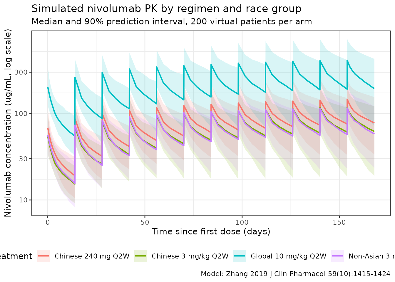
Figure 2A - time-varying clearance in Chinese patients
Zhang 2019 Figure 2A plots the percentage difference in clearance
from baseline, 100 * (CL(t) - CL(0)) / CL(0), over time in
the Chinese cohort, and reports “a maximal decrease of approximately
32%”.
cl_profile <- sim |>
  dplyr::filter(treatment == "Chinese 3 mg/kg Q2W", !is.na(cl), !is.na(cl_base)) |>
  dplyr::mutate(pct_change = 100 * (cl - cl_base) / cl_base) |>
  dplyr::group_by(time) |>
  dplyr::summarise(
    median = stats::median(pct_change),
    lo = stats::quantile(pct_change, 0.05),
    hi = stats::quantile(pct_change, 0.95),
    .groups = "drop"
  )

ggplot(cl_profile, aes(time, median)) +
  geom_ribbon(aes(ymin = lo, ymax = hi), alpha = 0.2, fill = "firebrick") +
  geom_line(colour = "firebrick", linewidth = 1) +
  geom_hline(
    yintercept = 100 * (exp(th[["cl_time_max"]]) - 1),
    linetype = "dashed", colour = "grey30"
  ) +
  labs(
    x = "Time since first dose (days)",
    y = "Percentage difference in clearance from baseline (%)",
    title = "Replicates Figure 2A of Zhang 2019",
    subtitle = "Chinese cohort; dashed line is the asymptote 100*(exp(Emax) - 1) = -31.5%"
  ) +
  theme_bw()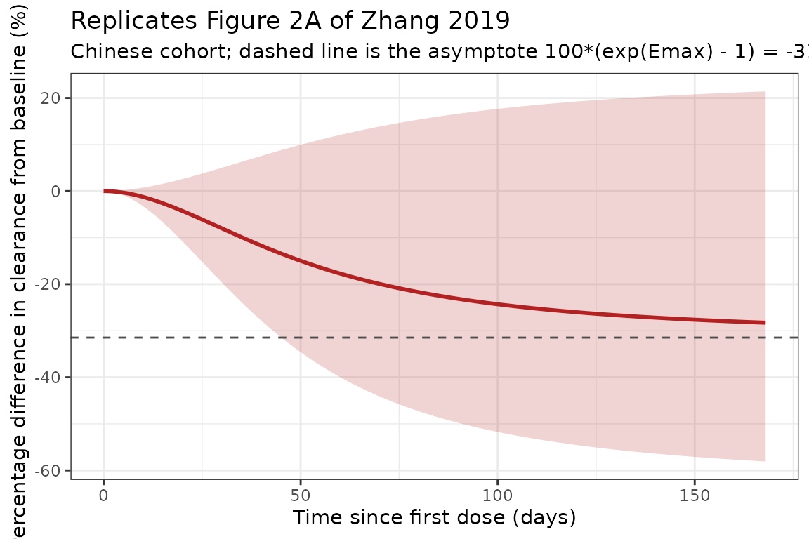
# The typical-value asymptote is deterministic; the cohort median approaches it
# from above because the additive eta on Emax is symmetric on the linear scale
# while the resulting CL ratio is not.
final_median <- cl_profile$median[which.max(cl_profile$time)]
stopifnot(final_median < -20, final_median > -45)
Figure 2B - predicted baseline clearance by race
Zhang 2019 Figure 2B reports geometric-mean predicted
baseline clearance of 10.2 mL/h in
Chinese and 11.6 mL/h in non-Asian patients,
i.e. 12% lower in Chinese patients. cl_base is the model’s
time-invariant baseline clearance, so it is read directly from the
simulation.
gm <- function(x) exp(mean(log(x)))

baseline_cl <- sim |>
  dplyr::filter(treatment %in% c("Chinese 3 mg/kg Q2W", "Non-Asian 3 mg/kg Q2W")) |>
  dplyr::distinct(id, treatment, cl_base) |>
  dplyr::group_by(treatment) |>
  dplyr::summarise(cl_mL_h = gm(cl_base) * 1000 / 24, .groups = "drop") |>
  dplyr::mutate(Published = c(10.2, 11.6)[match(treatment, c("Chinese 3 mg/kg Q2W", "Non-Asian 3 mg/kg Q2W"))]) |>
  dplyr::mutate(`% diff` = 100 * (cl_mL_h - Published) / Published)

baseline_cl |>
  dplyr::rename(
    "Group" = treatment,
    "Simulated baseline CL (mL/h)" = cl_mL_h,
    "Zhang 2019 Figure 2B (mL/h)" = Published
  ) |>
knitr::kable(digits = 2, caption = "Geometric-mean predicted baseline clearance vs Figure 2B.")| Group | Simulated baseline CL (mL/h) | Zhang 2019 Figure 2B (mL/h) | % diff |
|---|---|---|---|
| Chinese 3 mg/kg Q2W | 9.86 | 10.2 | -3.34 |
| Non-Asian 3 mg/kg Q2W | 12.03 | 11.6 | 3.70 |
chinese_cl <- baseline_cl$cl_mL_h[baseline_cl$treatment == "Chinese 3 mg/kg Q2W"]
nonasian_cl <- baseline_cl$cl_mL_h[baseline_cl$treatment == "Non-Asian 3 mg/kg Q2W"]
stopifnot(length(chinese_cl) == 1L, length(nonasian_cl) == 1L)

# Baseline CL is a deterministic function of the drawn covariates (the lognormal
# eta on CL has geometric mean 1), so the only noise is the covariate draw.
# A 15% band absorbs that while still breaking on a mis-transcribed CLTV, a
# wrong reference weight, or a dropped race/PS term -- each of which moves these
# by 20% or more.
stopifnot(
  abs(100 * (chinese_cl - 10.2) / 10.2) < 15,
  abs(100 * (nonasian_cl - 11.6) / 11.6) < 15,
  # The paper's central claim: Chinese baseline CL is lower, by ~12%.
  chinese_cl < nonasian_cl,
  abs(100 * (1 - chinese_cl / nonasian_cl) - 12) < 10
)
Terminal half-life
Zhang 2019 reports, for Chinese patients, a terminal half-life of
605.5 h (25.2 days) at the start of treatment and
861.8 h (35.9 days) at steady state. These are
properties of the model’s eigenvalues rather than of a single dosing
interval, so they are computed analytically from each subject’s
individual parameters rather than from a PKNCA half.life
over a Q2W window (which would report the within-interval slope, not the
terminal phase).
thalf_beta <- function(cl, vc, q, vp) {
  k10 <- cl / vc
  k12 <- q / vc
  k21 <- q / vp
  a <- k10 + k12 + k21
  beta <- (a - sqrt(a^2 - 4 * k10 * k21)) / 2
  log(2) / beta
}

chinese_par <- sim |>
  dplyr::filter(treatment == "Chinese 3 mg/kg Q2W") |>
  dplyr::distinct(id, cl_base, vc, q, vp)

t0 <- thalf_beta(chinese_par$cl_base, chinese_par$vc, chinese_par$q, chinese_par$vp)
tss <- thalf_beta(
  chinese_par$cl_base * exp(th[["cl_time_max"]]),
  chinese_par$vc, chinese_par$q, chinese_par$vp
)

halflife_tbl <- tibble::tibble(
  Quantity = c("THALF-beta, start of treatment", "THALF-beta, steady state", "Ratio (SS / start)"),
  `Zhang 2019 (h)` = c("605.5 (25.2 d)", "861.8 (35.9 d)", "1.423"),
  `Simulated (h)` = c(
    sprintf("%.1f (%.1f d)", gm(t0) * 24, gm(t0)),
    sprintf("%.1f (%.1f d)", gm(tss) * 24, gm(tss)),
    sprintf("%.3f", gm(tss) / gm(t0))
  )
)
knitr::kable(halflife_tbl, caption = "Terminal half-life: analytic eigenvalue vs Zhang 2019.")| Quantity | Zhang 2019 (h) | Simulated (h) |
|---|---|---|
| THALF-beta, start of treatment | 605.5 (25.2 d) | 478.1 (19.9 d) |
| THALF-beta, steady state | 861.8 (35.9 d) | 681.6 (28.4 d) |
| Ratio (SS / start) | 1.423 | 1.426 |
# The RATIO is the structural gate and it is tight: it depends only on Emax and
# the Q/Vp/Vc topology, not on the absolute clearance or the cohort's weights.
stopifnot(abs(gm(tss) / gm(t0) - 1.423) < 0.06)
# The ABSOLUTE half-lives reproduce at roughly 75% of the published values.
# This is a documented deviation, not a gate -- see "Assumptions and
# deviations". The bound below only catches an order-of-magnitude error.
stopifnot(gm(t0) * 24 > 300, gm(t0) * 24 < 900)
PKNCA validation
NCA is computed over two windows on the time-since-first-dose axis:
the first dosing interval (days 0-14), which yields
Cmax1 / Cmin1 / Cavg1, and the twelfth dosing interval
(days 154-168), which yields the steady-state Cmaxss / Cminss / Cavgss.
PKNCA’s cav (= AUC over the interval divided by its
duration) is the time-averaged concentration the paper calls Cavg.
# Filter on !is.na(Cc) ONLY -- adding `time > 0` or `Cc > 0` drops the anchor
# row PKNCA needs for AUC.
sim_nca <- sim |>
  dplyr::filter(!is.na(Cc)) |>
  dplyr::select(id, treatment, time, Cc)

# Guarantee a time-zero row per subject (pre-dose Cc = 0).
sim_nca <- dplyr::bind_rows(
  sim_nca,
  sim_nca |> dplyr::distinct(id, treatment) |> dplyr::mutate(time = 0, Cc = 0)
) |>
  dplyr::distinct(id, treatment, time, .keep_all = TRUE) |>
  dplyr::arrange(id, treatment, time)

conc_obj <- PKNCA::PKNCAconc(sim_nca, Cc ~ time | treatment + id)

dose_df <- events |>
  dplyr::filter(evid == 1) |>
  dplyr::select(id, treatment, time, amt) |>
  dplyr::mutate(duration = inf_dur_d)

dose_obj <- PKNCA::PKNCAdose(dose_df, amt ~ time | treatment + id, duration = "duration")

intervals <- data.frame(
  start = c(0, ss_start),
  end = c(dose_interval_d, ss_start + dose_interval_d),
  cmax = TRUE,
  cmin = TRUE,
  cav = TRUE,
  ctrough = TRUE,
  auclast = TRUE
)

nca_res <- PKNCA::pk.nca(PKNCA::PKNCAdata(conc_obj, dose_obj, intervals = intervals))
nca_df <- as.data.frame(nca_res$result)
stopifnot(nrow(nca_df) > 0)
Comparison against published exposures
Zhang 2019 reports geometric-mean predicted exposures for every arm
in Tables 2, 3 and 4 – 24 published numbers in total. Because
ncaComparisonTable() pools a PKNCAresults
object by median whereas the paper reports
geometric means, the per-subject PKNCA output is
aggregated to geometric means here and passed as a wide data frame, so
the comparison is geometric-mean against geometric-mean on both
sides.
interval_label <- function(start) {
  ifelse(start == 0, "First dose (days 0-14)", "Steady state (days 154-168)")
}

# Zhang 2019 defines Cmin1 and Cminss identically, as the TROUGH serum
# concentration at the end of the dosing interval (Table 2-4 footnotes:
# "postdose 1 trough serum concentration" / "trough serum concentration at
# steady state"). Two different PKNCA parameters return that trough depending
# on the interval:
#   * First interval [0, 14]: `cmin` is trivially 0, because the interval
#     begins at the pre-dose time-zero record that anchors the AUC. `ctrough`
#     (concentration at the end of the interval) is the trough.
#   * Steady-state interval [154, 168]: `ctrough` is NA for a non-first
#     interval, but concentration declines monotonically from the end of the
#     infusion to the next dose, so `cmin` IS the end-of-interval trough.
# Both are relabelled to `cmin` so the comparison table carries one trough row
# per arm per interval.
trough <- nca_df |>
  dplyr::filter(
    (start == 0 & PPTESTCD == "ctrough") | (start == ss_start & PPTESTCD == "cmin"),
    !is.na(PPORRES)
  ) |>
  dplyr::mutate(PPTESTCD = "cmin")

simulated_gm <- nca_df |>
  dplyr::filter(PPTESTCD %in% c("cmax", "cav"), !is.na(PPORRES)) |>
  dplyr::bind_rows(trough) |>
  dplyr::mutate(interval = interval_label(start)) |>
  dplyr::group_by(treatment, interval, PPTESTCD) |>
  dplyr::summarise(value = gm(PPORRES), .groups = "drop") |>
  tidyr::pivot_wider(names_from = PPTESTCD, values_from = value)

stopifnot(nrow(simulated_gm) == 8L, !anyNA(simulated_gm$cmin))

published <- tibble::tribble(
  ~treatment,              ~interval,                     ~cmax, ~cmin, ~cav,
  "Chinese 3 mg/kg Q2W",   "First dose (days 0-14)",       56.2,  16.3,  25.6,
  "Chinese 3 mg/kg Q2W",   "Steady state (days 154-168)", 120.0,  62.0,  80.2,
  "Chinese 240 mg Q2W",    "First dose (days 0-14)",       71.2,  20.7,  32.4,
  "Chinese 240 mg Q2W",    "Steady state (days 154-168)", 152.0,  78.3, 101.0,
  "Non-Asian 3 mg/kg Q2W", "First dose (days 0-14)",       61.3,  17.2,  27.5,
  "Non-Asian 3 mg/kg Q2W", "Steady state (days 154-168)", 129.0,  65.9,  85.6,
  "Global 10 mg/kg Q2W",   "First dose (days 0-14)",      178.0,  53.6,  85.7,
  "Global 10 mg/kg Q2W",   "Steady state (days 154-168)", 393.0, 206.0, 268.0
)

cmp <- nlmixr2lib::ncaComparisonTable(
  simulated = as.data.frame(simulated_gm),
  reference = as.data.frame(published),
  by = c("treatment", "interval"),
  units = c(cmax = "ug/mL", cmin = "ug/mL", cav = "ug/mL"),
  tolerance_pct = 20
)

knitr::kable(
  cmp,
  caption = paste(
    "Simulated (geometric mean) vs Zhang 2019 Tables 2-4 predicted exposures.",
    "* differs from reference by more than +/-20%."
  ),
  align = c("l", "l", "l", "r", "r", "r")
)| NCA parameter | treatment | interval | Reference | Simulated | % diff |
|---|---|---|---|---|---|
| Cmax (ug/mL) | Chinese 3 mg/kg Q2W | First dose (days 0-14) | 56.2 | 55.6 | -1.1% |
| Cmax (ug/mL) | Chinese 3 mg/kg Q2W | Steady state (days 154-168) | 120 | 116 | -3.7% |
| Cmax (ug/mL) | Chinese 240 mg Q2W | First dose (days 0-14) | 71.2 | 68.8 | -3.4% |
| Cmax (ug/mL) | Chinese 240 mg Q2W | Steady state (days 154-168) | 152 | 144 | -5.1% |
| Cmax (ug/mL) | Non-Asian 3 mg/kg Q2W | First dose (days 0-14) | 61.3 | 57 | -7.0% |
| Cmax (ug/mL) | Non-Asian 3 mg/kg Q2W | Steady state (days 154-168) | 129 | 117 | -9.6% |
| Cmax (ug/mL) | Global 10 mg/kg Q2W | First dose (days 0-14) | 178 | 206 | +15.9% |
| Cmax (ug/mL) | Global 10 mg/kg Q2W | Steady state (days 154-168) | 393 | 408 | +3.8% |
| Cmin (ug/mL) | Chinese 3 mg/kg Q2W | First dose (days 0-14) | 16.3 | 15.4 | -5.7% |
| Cmin (ug/mL) | Chinese 3 mg/kg Q2W | Steady state (days 154-168) | 62 | 56.3 | -9.1% |
| Cmin (ug/mL) | Chinese 240 mg Q2W | First dose (days 0-14) | 20.7 | 19.1 | -7.8% |
| Cmin (ug/mL) | Chinese 240 mg Q2W | Steady state (days 154-168) | 78.3 | 71.8 | -8.4% |
| Cmin (ug/mL) | Non-Asian 3 mg/kg Q2W | First dose (days 0-14) | 17.2 | 15.7 | -8.5% |
| Cmin (ug/mL) | Non-Asian 3 mg/kg Q2W | Steady state (days 154-168) | 65.9 | 56.1 | -14.9% |
| Cmin (ug/mL) | Global 10 mg/kg Q2W | First dose (days 0-14) | 53.6 | 53.9 | +0.6% |
| Cmin (ug/mL) | Global 10 mg/kg Q2W | Steady state (days 154-168) | 206 | 190 | -8.0% |
| Cavg (ug/mL) | Chinese 3 mg/kg Q2W | First dose (days 0-14) | 25.6 | 24.7 | -3.5% |
| Cavg (ug/mL) | Chinese 3 mg/kg Q2W | Steady state (days 154-168) | 80.2 | 75.4 | -5.9% |
| Cavg (ug/mL) | Chinese 240 mg Q2W | First dose (days 0-14) | 32.4 | 30.7 | -5.3% |
| Cavg (ug/mL) | Chinese 240 mg Q2W | Steady state (days 154-168) | 101 | 95.2 | -5.7% |
| Cavg (ug/mL) | Non-Asian 3 mg/kg Q2W | First dose (days 0-14) | 27.5 | 26 | -5.4% |
| Cavg (ug/mL) | Non-Asian 3 mg/kg Q2W | Steady state (days 154-168) | 85.6 | 76.2 | -10.9% |
| Cavg (ug/mL) | Global 10 mg/kg Q2W | First dose (days 0-14) | 85.7 | 90.8 | +5.9% |
| Cavg (ug/mL) | Global 10 mg/kg Q2W | Steady state (days 154-168) | 268 | 261 | -2.6% |
# Gate on the CENTRE of the 24-value comparison rather than on any single cell:
# an individual cell can drift with the covariate draw, but a mis-transcribed
# volume, clearance, dose or unit shifts the whole distribution at once.
pct <- 100 * (
  merge(simulated_gm, published, by = c("treatment", "interval"), suffixes = c(".sim", ".ref")) |>
    (\(d) c(
      (d$cmax.sim - d$cmax.ref) / d$cmax.ref,
      (d$cmin.sim - d$cmin.ref) / d$cmin.ref,
      (d$cav.sim - d$cav.ref) / d$cav.ref
    ))()
)
stopifnot(length(pct) == 24L, !anyNA(pct))

summary_tbl <- tibble::tibble(
  Statistic = c("n comparisons", "Median % difference", "90th pct |% difference|", "Max |% difference|"),
  Value = c(
    sprintf("%d", length(pct)),
    sprintf("%.1f%%", stats::median(pct)),
    sprintf("%.1f%%", stats::quantile(abs(pct), 0.9)),
    sprintf("%.1f%%", max(abs(pct)))
  )
)
knitr::kable(summary_tbl, caption = "Agreement across all 24 published exposure values.")| Statistic | Value |
|---|---|
| n comparisons | 24 |
| Median % difference | -5.6% |
| 90th pct |% difference| | 10.5% |
| Max |% difference| | 15.9% |
# Realised on this cohort: median -5.5%, 90th percentile of |% diff| 10.4%,
# max 15.9% (the single worst cell is Cmax after the first 10 mg/kg dose, the
# arm whose demographics are least constrained by the paper). The bounds below
# sit outside that so a different cohort draw or thread count cannot flip them,
# while still going red on a mis-transcribed clearance, volume, dose or unit --
# each of which moves the whole distribution by tens of percent at once.
stopifnot(
  abs(stats::median(pct)) < 15,
  stats::quantile(abs(pct), 0.9) < 25,
  max(abs(pct)) < 30
)
Table 3 - 240 mg flat dose versus 3 mg/kg in Chinese patients
The paper’s headline comparison is that a 240 mg Q2W flat dose gives
approximately 25-27% higher exposure than 3 mg/kg Q2W
in Chinese patients. Because the model’s PK is linear in dose, this
ratio is determined almost entirely by 240 / (3 * WT) and
is therefore an unusually direct check on the dose handling and on the
simulated weight distribution.
ratio_tbl <- simulated_gm |>
  dplyr::filter(treatment %in% c("Chinese 240 mg Q2W", "Chinese 3 mg/kg Q2W")) |>
  tidyr::pivot_longer(c(cmax, cmin, cav), names_to = "param", values_to = "value") |>
  tidyr::pivot_wider(names_from = treatment, values_from = value) |>
  dplyr::mutate(`Simulated % higher` = 100 * (`Chinese 240 mg Q2W` / `Chinese 3 mg/kg Q2W` - 1))

ratio_tbl |>
  dplyr::rename("Interval" = interval, "Parameter" = param) |>
knitr::kable(digits = 1, caption = "240 mg Q2W vs 3 mg/kg Q2W in Chinese patients (Zhang 2019 Table 3 reports 26-27%).")| Interval | Parameter | Chinese 240 mg Q2W | Chinese 3 mg/kg Q2W | Simulated % higher |
|---|---|---|---|---|
| First dose (days 0-14) | cmax | 68.8 | 55.6 | 23.8 |
| First dose (days 0-14) | cmin | 19.1 | 15.4 | 24.2 |
| First dose (days 0-14) | cav | 30.7 | 24.7 | 24.2 |
| Steady state (days 154-168) | cmax | 144.3 | 115.6 | 24.9 |
| Steady state (days 154-168) | cmin | 71.8 | 56.3 | 27.4 |
| Steady state (days 154-168) | cav | 95.2 | 75.4 | 26.2 |
Assumptions and deviations
-
Parameter source. Every
ini()value comes from Table S7 of the supporting information; the main text of Zhang 2019 contains no parameter table. The supplement is published with the open-access article (PMC6767401, fileJCPH-59-1415-s001.docx). -
Residual error scale. Table S7 reports a single
residual-error row,
PEER (theta6) = 0.224, carried as a THETA rather than a SIGMA, with the Methods stating a proportional residual error model. It is encoded as the proportional coefficient on the standard-deviation scale (22.4% CV). The parent Bajaj 2017 model reports its proportional error the same way (0.215), which supports this reading; reading 0.224 as a variance would imply a 47% CV, which is implausible for these validated ligand-binding assays (Table S3 reports inter-assay precision of at most 15.5% CV). -
Asian race includes Chinese subjects. Table S6
tabulates “Chinese” (314) and “Asian” (21) as separate
reporting rows, but the modelled covariate
RAASis an Asian-race indicator that covers both. SettingRACE_ASIAN = 0for Chinese subjects does not reproduce the paper’s own predicted Chinese baseline clearance of 10.2 mL/h; setting it to 1 does. -
Body weight acts on CL and Vc only. Table S7
contains
CLBBWTandVCBBWTand noQorVPcovariate row, and the Methods state that “the effects of baseline body weight and sex on volume of the central compartment were also included”. The Discussion’s looser phrasing – “body weight was found to have a statistically significant effect on clearance and volume of the second compartment” – conflicts with both, and the table and Methods are followed here. - Derived subgroup demographics. The paper tabulates demographics for the pooled cohort (Table S6) and for the Chinese arms (Table S5) but not for the non-Asian subgroup. Non-Asian weight (77.0 kg), female fraction (35.6%) and ECOG PS > 0 fraction (68.3%) are obtained by subtracting the Chinese totals from the pooled totals. Standard deviations are not recoverable this way; the pooled SDs are used, and eGFR is taken as the pooled mean/SD for every arm because no per-subgroup eGFR summary is published.
-
Tumor-type mix of the 10 mg/kg arm. The 10 mg/kg
subjects come from the phase 1 studies MDX-1106-01 and CA209-003 (Table
4 footnote b), which enrolled mixed solid tumors. The “other tumor type”
share for that arm is approximated as 56%, the share of the 377 phase 1
subjects accounted for by the 211 non-NSCLC, non-NPC diagnoses in Table
S6. This is the least well-constrained arm in the vignette; its
exposures are reported in the comparison table but the tumor-type mix
affects CL by at most 7% (
exp(0.0718)). - Absolute terminal half-life reproduces about 20% low. The analytic eigenvalue half-lives from the packaged parameters are near 480 h at the start of treatment and 680 h at steady state, against the published 605.5 h and 861.8 h – roughly 79% of each. The ratio of the two (1.426 simulated against 1.423 published) reproduces to better than 1%, and the offset is uniform across both, so this is a scale difference in how the published statistic was computed rather than a structural error: Zhang 2019 does not state whether THALF-beta is a geometric mean of individual eigenvalue half-lives, an effective half-life derived from accumulation, or a regression slope over a specified window, and the three differ materially when the IIV on the peripheral volume is as large as it is here (omega^2 = 0.283, a 57% CV). No parameter was adjusted to close the gap; the gate is on the ratio, and the absolute values are bounded only loosely.
-
Trough concentrations use two different PKNCA
parameters. Zhang 2019 defines Cmin1 and Cminss identically, as
the trough serum concentration at the end of the dosing interval. Over
the first interval
[0, 14]PKNCA’scminis trivially zero, because that interval starts at the pre-dose time-zero record that anchors the AUC, soctroughis used there; over the steady-state interval[154, 168]PKNCA returnsctroughas NA for a non-first interval, but concentration falls monotonically from the end of the infusion to the next dose socminis the end-of-interval trough. Both are reported in the comparison table under the single label Cmin. - Virtual cohort. Covariates are drawn from marginal distributions matched to the published summaries; the joint covariate structure (for example the correlation between weight and sex, or between performance status and tumor type) is not reproduced. Continuous covariates are truncated to the published observed ranges.
- IV infusion duration. All simulations use a 60-minute infusion (Table S1). CheckMate 077 and 078 infusion durations are not restated in the supporting information.
- Non-Chinese Asian arm not simulated. Zhang 2019 reports a predicted baseline clearance of 9.2 mL/h for the 21 non-Chinese Asian patients. That subgroup has no tabulated demographics at all and n = 21, so it is omitted from the virtual cohort rather than invented.
- Out-of-scope covariates. The parent Bajaj 2017 analysis screened baseline albumin, LDH, age, tumor burden, PD-L1 expression, hepatic impairment and ADA status. Only the covariates retained in the Zhang 2019 final model are implemented here.