Diclazuril PBPK in broiler chickens (Yang 2023)
Source:vignettes/articles/Yang_2023_diclazuril.Rmd
Yang_2023_diclazuril.RmdModel and source
- Citation: Yang F, Zhang M, Jin Y-G, Chen J-C, Duan M-H, Liu Y, Li Z-E, Li X-P, Yang F. Development and Application of a Physiologically Based Pharmacokinetic Model for Diclazuril in Broiler Chickens. Animals (Basel). 2023;13(9):1512. doi:10.3390/ani13091512
- Description: PBPK (whole-body, flow-limited; broiler chicken). Nine-compartment physiologically based pharmacokinetic model for the anticoccidial diclazuril in broiler chickens after continuous oral exposure via medicated feed or drinking water, comprising intestinal contents (absorption site), liver, kidney, lumped skin + fat, muscle, a lumped rest-of-body compartment, lung, arterial plasma and venous plasma; all tissues are perfusion (flow) limited with tissue:plasma partition coefficients, absorption from the gut lumen is first order (Ka) in competition with first-order fecal loss of unabsorbed drug (Kgut), and elimination is hepatic (Clhe) plus fecal excretion. Built to predict edible-tissue residues and withdrawal periods against Chinese and European maximum residue limits (Yang 2023).
- Article: https://doi.org/10.3390/ani13091512
- Supplement (acslX model code, M-file, Figures S1-S11): https://www.mdpi.com/article/10.3390/ani13091512/s1
Yang 2023 is the first physiologically based pharmacokinetic (PBPK) model for the anticoccidial diclazuril in broiler chickens. Its purpose is regulatory: predict diclazuril residues in edible tissues after continuous medicated-feed or medicated-water exposure, and from those predictions derive a withdrawal period against the Chinese and European maximum residue limits (MRLs).
The model is a nine-compartment, flow-limited
(perfusion-limited) whole-body PBPK model: intestinal contents (the site
of exposure and absorption), liver, kidney, lumped skin + fat, muscle, a
lumped rest-of-body compartment, lung, arterial plasma and venous
plasma. Absorption from the gut lumen is first order (Ka)
and competes with first-order fecal loss of unabsorbed drug
(Kgut); elimination is hepatic (Clhe) plus
that fecal route.
Population
The model was built from five concentration-time datasets in four published broiler studies (Yang 2023 Table 1) rather than from a single trial: three sets were used for parameter optimisation and two were held back for external validation. Birds were Lingnan Yellow Chickens and Ross 308 broilers, 15-50 days old, with study mean body weights of 1.23-1.52 kg – all close to market age, so Yang 2023 held body weight constant through each simulation. Exposure routes span single oral gavage (80 ug/kg BW and 1 mg/kg BW), medicated feed (730 ug/kg and 1 mg/kg) and medicated water (0.5-1 mg/L recommended; 3 mg/L in one validation study), given for 7-10 consecutive days.
Because chickens stop eating and drinking in the dark, the light regime sets the daily exposure window: 12/12 h for refs [1,19,20], 21/3 h for ref [22] and 18/6 h for ref [21]. Yang 2023 assumed a daily intake of 1.1 kg feed and 0.5 L water per bird spread evenly over the light hours.
Physiological parameters are broiler population means from the Wang et al. 2020 food-animal physiology review (Yang 2023 ref [24]). No individual-level data were fitted, so the model carries no inter-individual random effects; Yang 2023 instead propagated parameter uncertainty through a 1000-iteration Monte Carlo analysis over the normal distributions in its Table 4.
The same information is available programmatically via the model’s
population metadata
(readModelDb("Yang_2023_diclazuril_chicken_pbpk")()$population).
Source trace
Per-parameter provenance is recorded as an in-file comment next to
each ini() entry (and next to each physiological literal in
model()) in
inst/modeldb/specificDrugs/Yang_2023_diclazuril_chicken_pbpk.R.
Collected here for review:
| Equation / parameter | Value | Source location |
|---|---|---|
co (cardiac output) |
9.88 L/h/kg | Table 3 footnote 2; supplement constant CO=9.88
|
pcv (hematocrit) |
0.32 | Section 2.3 (“32 +/- 2.76%”); supplement
constant pcv=0.32
|
vc_muscle |
0.5712 | Table 3; supplement constant vcmu
|
vc_liver |
0.0214 | Table 3; supplement constant vcli
|
vc_kidney |
0.0064 | Table 3; supplement constant vcki
|
vc_lung |
0.0071 | Table 3; supplement constant vclu
|
vc_blood |
0.0483 | Table 4 (Vcbl 4.83%); supplement
constant vcbl
|
vc_skin |
0.1338 | Table 4 (Vcsk 13.38%); supplement
constant vcsk
|
vc_fat |
0.134 | Table 4 (Vcfa 13.4%); supplement
constant vcfa
|
qc_muscle |
0.0764 | Table 3; supplement constant qcmu
|
qc_liver |
0.2526 | Table 3 + footnote 4 (hepatic artery + portal vein) |
qc_kidney |
0.2012 | Table 3; supplement constant qcki
|
qc_lung |
1.0 | Table 3 + footnote 6 (equals Qtot) |
qc_skin |
0.1505 | Supplement constant qcsk (Table 3 prints only the skin
+ fat sum) |
qc_fat |
0.1 | Supplement constant qcfa (Table 3 prints only the skin
+ fat sum) |
v_other, q_other
|
0.0778, 0.2193 | Table 3 footnotes 7 and 8 (balance of BW / of CO) |
lk_mus (Pmu) |
0.1299 | Table 3 / Section 3.1 (area method) |
lk_skf (Psf) |
0.0955 | Table 3 / Section 3.1 (area method) |
lk_kid (Pki) |
0.6813 | Table 3 / Section 3.1 (area method) |
lk_liv (Pli) |
0.9613 | Table 3 + footnote 5 / Section 3.1 (optimised) |
lk_lun (Plu) |
0.5603 | Table 3 + footnote 5 / Section 3.1 (optimised) |
lk_res (Pre) |
1.2965 | Table 3 + footnote 5 / Section 3.1 (optimised) |
lka (Ka) |
0.1234 1/h | Section 3.1 / Table 4 (optimised) |
lkgut (Kgut) |
0.3838 1/h | Section 3.1 / Table 4 (optimised) |
lclhe (Clhe) |
0.00344 L/h/kg | Section 3.1 / Table 4 (optimised) |
d/dt(a_gut) |
n/a | Table 2 “Intestinal contents”; supplement ragicon
|
d/dt(liver) |
n/a | Table 2 “Liver”; supplement rali
|
d/dt(kidney) |
n/a | Table 2 “Kidney”; supplement raki
|
d/dt(skin_fat) |
n/a | Table 2 “Skin + fat”; supplement rasf
|
d/dt(muscle) |
n/a | Table 2 “Muscle”; supplement ramu
|
d/dt(other) |
n/a | Table 2 “Rest”; supplement rare
|
d/dt(lung) |
n/a | Table 2 “Lung”; supplement ralu
|
d/dt(arterial) |
n/a | Table 2 “Arterial plasma”; supplement raap
|
d/dt(venous) |
n/a | Table 2 “Venous plasma”; supplement ravp
|
| Bioavailability 24.32% | n/a | Section 3.1 / Section 4 |
| MRLs (China / Europe) | see below | Section 1 (Introduction); supplement M-file |
| Observed gavage Tmax 29.1-34.3 h | n/a | Section 4 (Discussion) |
propSd* are not paper-derived – see
Assumptions and deviations.
Exposure scenarios
Diclazuril is not given as a discrete bolus but eaten or drunk over
the daily light period. In the acslX source this is
dose/tlen * PULSE(...); here the daily dose is a
zero-order input into a_gut of duration
tlen hours, repeated every 24 h, so
tlen is a property of the event table rather than of the
model. The daily dose is the diclazuril concentration in feed or water
times the assumed daily intake (1.1 kg feed or 0.5 L water).
Every simulation below is a typical-value (deterministic) prediction:
the model has no random effects, so one bird per scenario is sufficient
and no zeroRe() step is needed.
# Daily dose (ug/day) = concentration in feed/water * daily intake.
feed_per_day  <- 1.1   # kg/day  (Yang 2023 Section 2.2)
water_per_day <- 0.5   # L/day   (Yang 2023 Section 2.2)

# Build one continuous-exposure scenario as a self-contained event table.
# `tlen` is the daily light period; `n_days` the number of dosing days.
make_scenario <- function(id, label, dose_per_day, tlen, n_days, wt, obs_h) {
  rxode2::et(amt = dose_per_day, dur = tlen, ii = 24,
             until = 24 * (n_days - 1), cmt = "a_gut") |>
    rxode2::et(seq(0, obs_h, by = 1), cmt = "venous") |>
    as.data.frame() |>
    dplyr::mutate(
      id = id, WT = wt, scenario = label,
      # Six-endpoint model: observation rows point at the ODE state
      # (`venous`) and carry an explicit dvid. rxode2 returns every
      # algebraic observable as a column regardless of the dvid chosen.
      dvid = ifelse(evid == 0, 1L, NA_integer_)
    )
}

scenarios <- dplyr::bind_rows(
  # External-validation datasets (Yang 2023 Figures 2 and 3).
  make_scenario(1L, "Feed 730 ug/kg, 10 d",  0.730 * feed_per_day  * 1000,
                tlen = 21, n_days = 10, wt = 1.50, obs_h = 24 * 20),
  make_scenario(2L, "Water 3 mg/L, 9 d",     3.0   * water_per_day * 1000,
                tlen = 12, n_days =  9, wt = 1.34, obs_h = 24 * 20),
  # The two label-recommended regimens (Yang 2023 Section 2.6).
  make_scenario(3L, "Feed 1 mg/kg, 20 d",    1.0   * feed_per_day  * 1000,
                tlen = 12, n_days = 20, wt = 1.50, obs_h = 24 * 26),
  make_scenario(4L, "Water 1 mg/L, 20 d",    1.0   * water_per_day * 1000,
                tlen = 12, n_days = 20, wt = 1.50, obs_h = 24 * 26)
)

stopifnot(!anyDuplicated(unique(scenarios[, c("id", "time", "evid")])))

mod <- rxode2::rxode(readModelDb("Yang_2023_diclazuril_chicken_pbpk"))
sim <- rxode2::rxSolve(mod, events = scenarios,
                       keep = c("WT", "scenario"),
                       returnType = "data.frame", addDosing = FALSE)
#> Warning: multi-subject simulation without without 'omega'
Regulatory limits used throughout (Yang 2023 Introduction; the Chinese values are also hard-coded in the supplement’s M-file):
mrl <- tibble::tribble(
  ~tissue,      ~china, ~europe,
  "Muscle",        500,     500,
  "Skin + fat",   1000,     500,
  "Kidney",       2000,    1000,
  "Liver",        3000,    1500
)
knitr::kable(
  mrl |> dplyr::rename("Tissue" = tissue,
                       "China MRL (ug/kg)" = china,
                       "Europe MRL (ug/kg)" = europe),
  caption = "Diclazuril maximum residue limits (Yang 2023 Introduction)."
)| Tissue | China MRL (ug/kg) | Europe MRL (ug/kg) |
|---|---|---|
| Muscle | 500 | 500 |
| Skin + fat | 1000 | 500 |
| Kidney | 2000 | 1000 |
| Liver | 3000 | 1500 |
Structural verification
Before comparing against published figures, four checks confirm the ODE system was transcribed correctly.
1. Dimensional analysis
Each tissue equation has the form
V_i * dC_i/dt = Q_i * (C_art - C_i / P_i), and the packaged
model integrates amounts (ug), exactly as the
supplement does. Units therefore reconcile as
L/h * ug/L = ug/h on the right-hand side against
d(ug)/dt on the left. The hepatic loss term is
Clhe [L/h/kg] * WT [kg] * C_li/P_li [ug/L] = ug/h, and
absorption is Ka [1/h] * A_gut [ug] = ug/h. Concentrations
in tissue are reported as ug/kg and in plasma as ug/L, with tissue
density taken as 1 kg/L.
2. Steady-state tissue:plasma ratios recover the partition coefficients
In a flow-limited model, once distribution has equilibrated each
tissue concentration approaches P_i times the arterial
plasma concentration. This is the sharpest available test of the
distribution block.
ss <- sim |>
  dplyr::filter(scenario == "Feed 1 mg/kg, 20 d",
                dplyr::near(time, 24 * 24)) |>   # 4 days after the last dose
  dplyr::slice(1)

ratio_check <- tibble::tibble(
  Tissue    = c("Muscle", "Skin + fat", "Kidney", "Liver", "Lung"),
  Published = c(0.1299, 0.0955, 0.6813, 0.9613, 0.5603),
  Model     = c(ss$Cmuscle, ss$Cskin_fat, ss$Ckidney, ss$Cliver, ss$Clung) / ss$Cc
) |>
  dplyr::mutate(`Percent difference` = 100 * (Model - Published) / Published)

knitr::kable(ratio_check, digits = c(0, 4, 4, 2),
             caption = paste("Simulated tissue:plasma concentration ratio vs the",
"published partition coefficients of Yang 2023 Table 3."))| Tissue | Published | Model | Percent difference |
|---|---|---|---|
| Muscle | 0.1299 | 0.1301 | 0.13 |
| Skin + fat | 0.0955 | 0.0955 | 0.02 |
| Kidney | 0.6813 | 0.6813 | 0.00 |
| Liver | 0.9613 | 0.9601 | -0.12 |
| Lung | 0.5603 | 0.5603 | 0.00 |
3. Absolute bioavailability
Unabsorbed drug leaves the gut lumen only by absorption
(Ka) or defecation (Kgut), so whatever the
dosing history the absorbed fraction is the closed form
Ka / (Ka + Kgut). Yang 2023 computed 24.32% numerically as
the ratio of total absorbed to total administered (Section 3.1).
4. Mass balance
Total administered drug must equal drug still in the body plus drug lost by the two elimination routes. Fecal and hepatic losses are recovered by integrating the simulated profiles (the packaged model carries no cumulative-loss states).
mb_one <- function(df, dose_per_day, n_days, wt) {
  df <- dplyr::arrange(df, time)
  trap <- function(y) sum(diff(df$time) * (utils::head(y, -1) + utils::tail(y, -1)) / 2)
  in_body <- with(df, a_gut + liver + kidney + skin_fat + muscle + other +
                    lung + arterial + venous)
  fecal   <- kgut * trap(df$a_gut)
  hepatic <- exp(p[["lclhe"]]) * wt * trap(df$Cliver / exp(p[["lk_liv"]]))
  dosed   <- dose_per_day * n_days
  tibble::tibble(
    Dosed = dosed, `In body` = utils::tail(in_body, 1),
    Fecal = fecal, Hepatic = hepatic,
    `Balance (% of dose)` =
      100 * (dosed - utils::tail(in_body, 1) - fecal - hepatic) / dosed
  )
}

mb <- dplyr::bind_rows(
  mb_one(dplyr::filter(sim, scenario == "Water 3 mg/L, 9 d"),
         3.0 * water_per_day * 1000, 9, 1.34) |>
    dplyr::mutate(Scenario = "Water 3 mg/L, 9 d", .before = 1),
  mb_one(dplyr::filter(sim, scenario == "Feed 1 mg/kg, 20 d"),
         1.0 * feed_per_day * 1000, 20, 1.50) |>
    dplyr::mutate(Scenario = "Feed 1 mg/kg, 20 d", .before = 1)
)
knitr::kable(mb, digits = 2,
caption = "Mass balance: administered vs retained plus eliminated (ug).")| Scenario | Dosed | In body | Fecal | Hepatic | Balance (% of dose) |
|---|---|---|---|---|---|
| Water 3 mg/L, 9 d | 13500 | 32.61 | 10215.49 | 3251.89 | 0 |
| Feed 1 mg/kg, 20 d | 22000 | 122.01 | 16647.47 | 5230.51 | 0 |
The balance closes to 0.00% of the administered dose in both
scenarios: nothing leaks from the ODE system, and essentially all drug
has left the bird by the end of the observation window. Fecal excretion
of unabsorbed drug accounts for about three quarters of the dose and
hepatic metabolism the remainder, matching the closed-form split
Kgut / (Ka + Kgut) = 75.7% – and confirming Yang 2023’s
conclusion that diclazuril “is primarily eliminated with feces, followed
by hepatic metabolism”.
Replicate published figures
Figure 2 – medicated feed, 730 ug/kg for 10 days
tissue_long <- function(df) {
  df |>
    dplyr::select(time, scenario, Cc, Cmuscle, Cliver, Ckidney, Cskin_fat) |>
    tidyr::pivot_longer(c(Cc, Cmuscle, Cliver, Ckidney, Cskin_fat),
                        names_to = "matrix", values_to = "conc") |>
    dplyr::mutate(matrix = dplyr::recode(matrix,
      Cc = "Plasma", Cmuscle = "Muscle", Cliver = "Liver",
      Ckidney = "Kidney", Cskin_fat = "Skin + fat"))
}

sim |>
  dplyr::filter(scenario == "Feed 730 ug/kg, 10 d") |>
  tissue_long() |>
  ggplot(aes(time / 24, conc)) +
  geom_line(linewidth = 0.7) +
  facet_wrap(~matrix, scales = "free_y") +
  labs(x = "Time (days)", y = "Diclazuril (ug/kg or ug/L)",
       title = "Medicated feed 730 ug/kg for 10 consecutive days",
       caption = "Replicates Figure 2 of Yang 2023 (Mortier et al. dataset, ref [22]).")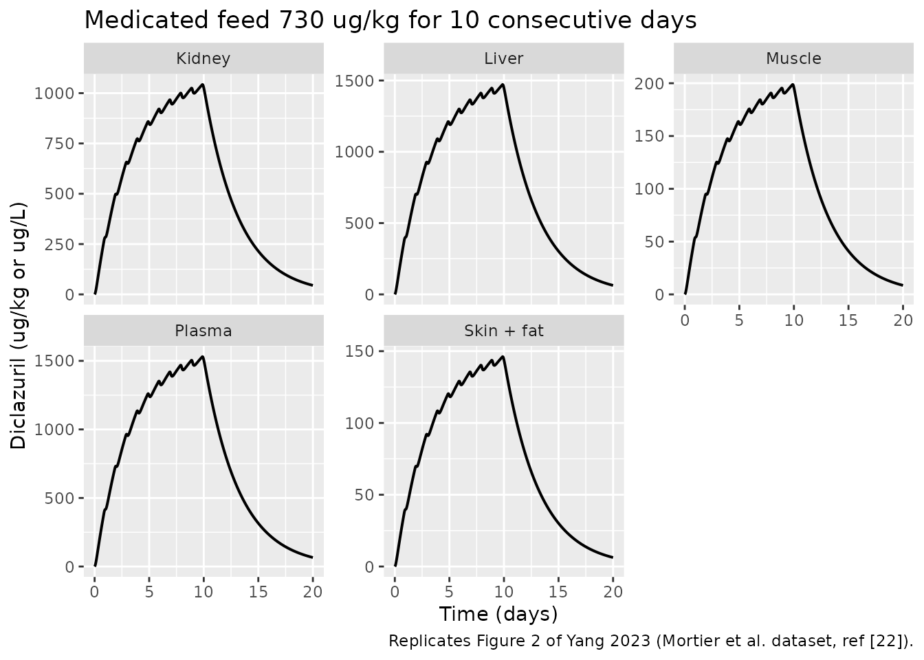
Dosing raises tissue concentrations to a plateau within the 10-day exposure and depletion begins as soon as the medicated feed is withdrawn, with liver the highest of the edible tissues and skin + fat the lowest – the ordering set by the partition coefficients and matching Figure 2 of Yang 2023.
Figure 3 – medicated water, 3 mg/L for 9 days
sim |>
  dplyr::filter(scenario == "Water 3 mg/L, 9 d") |>
  tissue_long() |>
  ggplot(aes(time / 24, conc)) +
  geom_line(linewidth = 0.7) +
  facet_wrap(~matrix, scales = "free_y") +
  labs(x = "Time (days)", y = "Diclazuril (ug/kg or ug/L)",
       title = "Medicated water 3 mg/L for 9 consecutive days",
       caption = "Replicates Figure 3 of Yang 2023 (Wen et al. dataset, ref [20]).")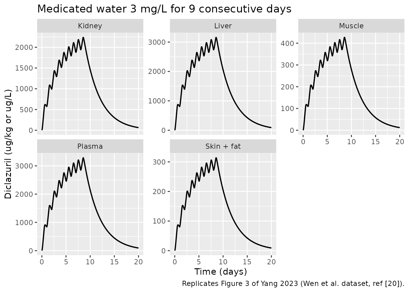
Steady state is reached by about 15 days (Figures S2-S9)
Yang 2023 reported that continuous exposure at the recommended levels reaches steady state after 15 days, so a 20-day exposure bounds the worst case.
sim |>
  dplyr::filter(scenario %in% c("Feed 1 mg/kg, 20 d", "Water 1 mg/L, 20 d")) |>
  tissue_long() |>
  ggplot(aes(time / 24, conc, colour = scenario)) +
  geom_line(linewidth = 0.7) +
  geom_vline(xintercept = 15, linetype = "dotted") +
  facet_wrap(~matrix, scales = "free_y") +
  labs(x = "Time (days)", y = "Diclazuril (ug/kg or ug/L)", colour = NULL,
       title = "Recommended regimens, 20 consecutive days",
       caption = paste("Replicates Figures S5 and S9 of Yang 2023.",
                       "Dotted line marks day 15.")) +
  theme(legend.position = "bottom")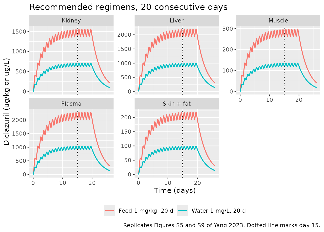
# Plateau check: how far is day 15 from day 20 at the end of exposure?
plateau <- sim |>
  dplyr::filter(scenario == "Feed 1 mg/kg, 20 d",
                time %in% c(24 * 15, 24 * 20)) |>
  dplyr::select(time, Cmuscle, Cliver, Ckidney, Cskin_fat) |>
  tidyr::pivot_longer(-time, names_to = "matrix", values_to = "conc") |>
  tidyr::pivot_wider(names_from = time, values_from = conc) |>
  dplyr::mutate(`Percent change, day 15 to 20` =
                  100 * (`480` - `360`) / `360`)
knitr::kable(plateau, digits = 2,
caption = "Approach to steady state under medicated feed at 1 mg/kg.")| matrix | 360 | 480 | Percent change, day 15 to 20 |
|---|---|---|---|
| Cmuscle | 263.36 | 265.25 | 0.72 |
| Cliver | 1943.98 | 1957.96 | 0.72 |
| Ckidney | 1379.53 | 1389.45 | 0.72 |
| Cskin_fat | 193.39 | 194.78 | 0.72 |
Withdrawal periods against the MRLs
The regulatory output of Yang 2023 is the withdrawal period: the time after the last dose at which every edible tissue sits below its MRL. Yang 2023 derived it from the 95th percentile of a 1000-bird Monte Carlo population; the packaged model reproduces the typical-bird value, which should be no longer than the 95th-percentile value.
withdrawal <- function(df, last_dose_end, limits) {
  post <- df |> dplyr::filter(time >= last_dose_end) |> dplyr::arrange(time)
  over <- with(post,
    Cmuscle   > limits[["Muscle"]]     |
    Cskin_fat > limits[["Skin + fat"]] |
    Ckidney   > limits[["Kidney"]]     |
    Cliver    > limits[["Liver"]])
  if (!any(over)) return(0)
  (post$time[max(which(over))] - last_dose_end) / 24
}

lim_cn <- setNames(mrl$china,  mrl$tissue)
lim_eu <- setNames(mrl$europe, mrl$tissue)

wt_tab <- tibble::tribble(
  ~Scenario,               ~end,
  "Feed 1 mg/kg, 20 d",    24 * 19 + 12,
  "Water 1 mg/L, 20 d",    24 * 19 + 12,
  "Water 3 mg/L, 9 d",     24 *  8 + 12
) |>
  dplyr::rowwise() |>
  dplyr::mutate(
    `China (days)`  = withdrawal(dplyr::filter(sim, scenario == Scenario), end, lim_cn),
    `Europe (days)` = withdrawal(dplyr::filter(sim, scenario == Scenario), end, lim_eu)
  ) |>
  dplyr::ungroup() |>
  dplyr::select(-end)

knitr::kable(wt_tab, caption = paste(
  "Typical-bird withdrawal period. Yang 2023 reports 0 days for both",
  "recommended regimens under the Chinese MRLs, and 1 day (China) /",
"4 days (Europe) for the 3 mg/L water regimen."))| Scenario | China (days) | Europe (days) |
|---|---|---|
| Feed 1 mg/kg, 20 d | 0.0000000 | 1.541667 |
| Water 1 mg/L, 20 d | 0.0000000 | 0.000000 |
| Water 3 mg/L, 9 d | 0.4583333 | 2.666667 |
Every published conclusion is reproduced, and in the right direction:
- Both recommended regimens clear all four Chinese MRLs immediately (0 days) – Yang 2023’s headline result.
- Medicated water at 1 mg/L also clears the European MRLs at 0 days, again matching Yang 2023, which found a 0-day European withdrawal for every water duration.
- Medicated feed at 1 mg/kg does not clear the European MRLs immediately: 1.54 days here versus the 1.65 days Yang 2023 reports for 20 days of feeding. This is the paper’s finding that “based on the European MRLs, longer periods were determined for the mediated feed dosing route” (0.63, 1.41, 1.63 and 1.65 days for 5, 10, 15 and 20 days).
- The above-label 3 mg/L water regimen breaches both MRL sets: 0.46 days (China) and 2.67 days (Europe) here, versus Yang 2023’s 1 day and 4 days.
The typical-bird values are consistently a little shorter than Yang 2023’s, which is the expected relationship – the published numbers are 95th-percentile withdrawal periods from a 1000-bird Monte Carlo population, so they must bound the typical bird from above.
peaks <- sim |>
  dplyr::filter(scenario == "Water 3 mg/L, 9 d") |>
  dplyr::summarise(Muscle = max(Cmuscle), `Skin + fat` = max(Cskin_fat),
                   Kidney = max(Ckidney), Liver = max(Cliver)) |>
  tidyr::pivot_longer(dplyr::everything(), names_to = "tissue",
                      values_to = "Peak (ug/kg)") |>
  dplyr::left_join(mrl, by = "tissue") |>
  dplyr::rename("Tissue" = tissue, "China MRL" = china, "Europe MRL" = europe)
knitr::kable(peaks, digits = 0, caption = paste(
  "Peak residues under medicated water at 3 mg/L vs the MRLs",
"(Yang 2023 Figure S11)."))| Tissue | Peak (ug/kg) | China MRL | Europe MRL |
|---|---|---|---|
| Muscle | 427 | 500 | 500 |
| Skin + fat | 314 | 1000 | 500 |
| Kidney | 2239 | 2000 | 1000 |
| Liver | 3160 | 3000 | 1500 |
PKNCA validation – single-gavage absorption
The continuous-exposure scenarios above have no washout to characterise, so NCA is applied to the single-gavage case instead. Yang 2023 notes in its Discussion that a single gavage dose produced peak plasma concentrations at 29.1 to 34.3 h, which it cites as evidence of slow diclazuril absorption. That observed Tmax range is the quantitative NCA target.
gavage <- rxode2::et(amt = 1.0 * 1.52 * 1000, dur = 0.001, cmt = "a_gut") |>
  rxode2::et(seq(0, 240, by = 0.5), cmt = "venous") |>
  as.data.frame() |>
  dplyr::mutate(id = 1L, WT = 1.52, treatment = "Single gavage 1 mg/kg BW",
                dvid = ifelse(evid == 0, 1L, NA_integer_))

sim_gav <- rxode2::rxSolve(mod, events = gavage, keep = c("WT", "treatment"),
                           returnType = "data.frame", addDosing = FALSE)

sim_nca <- sim_gav |>
  # A single-subject solve returns no `id` column; add it back for PKNCA.
  dplyr::mutate(id = 1L) |>
  dplyr::filter(!is.na(Cc)) |>
  dplyr::select(id, time, Cc, treatment)

# Guarantee a time-zero row (pre-dose Cc = 0 for extravascular dosing).
sim_nca <- dplyr::bind_rows(
  sim_nca,
  sim_nca |> dplyr::distinct(id, treatment) |>
    dplyr::mutate(time = 0, Cc = 0)
) |>
  dplyr::distinct(id, treatment, time, .keep_all = TRUE) |>
  dplyr::arrange(id, treatment, time)

conc_obj <- PKNCA::PKNCAconc(sim_nca, Cc ~ time | treatment + id)

dose_df <- gavage |>
  dplyr::filter(evid == 1) |>
  dplyr::select(id, time, amt, treatment)
dose_obj <- PKNCA::PKNCAdose(dose_df, amt ~ time | treatment + id,
                             route = "extravascular")

intervals <- data.frame(start = 0, end = Inf,
                        cmax = TRUE, tmax = TRUE,
                        aucinf.obs = TRUE, half.life = TRUE)

nca_res <- PKNCA::pk.nca(PKNCA::PKNCAdata(conc_obj, dose_obj,
                                          intervals = intervals))
Comparison against published values
published <- tibble::tibble(
  treatment = "Single gavage 1 mg/kg BW",
  tmax      = 31.7   # midpoint of the observed 29.1-34.3 h range (Yang 2023 Discussion)
)

cmp <- nlmixr2lib::ncaComparisonTable(
  simulated     = nca_res,
  reference     = published,
  by            = "treatment",
  units         = c(cmax = "ug/L", aucinf.obs = "ug*h/L",
                    tmax = "h", half.life = "h"),
  tolerance_pct = 20
)

knitr::kable(cmp, caption = paste(
  "Simulated vs published NCA after a single 1 mg/kg BW gavage dose.",
  "Only Tmax was reported by Yang 2023; Cmax, AUC and half-life are",
  "shown for completeness with no published counterpart.",
"* differs from reference by >20%."))| NCA parameter | treatment | Reference | Simulated | % diff |
|---|---|---|---|---|
| Tmax (h) | Single gavage 1 mg/kg BW | 31.7 | 7.5 | -76.3%* |
tmax_sim <- as.data.frame(nca_res) |>
  dplyr::filter(PPTESTCD == "tmax") |>
  dplyr::pull(PPORRES)
cat(sprintf("Simulated Tmax = %.1f h; Yang 2023 observed 29.1-34.3 h\n", tmax_sim))
#> Simulated Tmax = 7.5 h; Yang 2023 observed 29.1-34.3 h
This check fails, and the failure is a property of the
published model rather than of the transcription. The simulated
Tmax is about 7.5 h against an observed 29.1-34.3 h, a starred (>20%)
discrepancy. The reason is structural and can be read straight off the
parameters: unabsorbed drug leaves the gut lumen at
Ka + Kgut = 0.1234 + 0.3838 = 0.5072 1/h, a lumen half-life
of only 1.4 h, so the absorption input is essentially finished within ~7
h and plasma must peak there. Ka alone is slow, but it is
not what sets the input duration – the sum is, because
Kgut competes for the same pool (Yang 2023 Table 2,
dA_ic/dt = dose/tlen - Ka*A_ic - Kgut*A_ic). No
parameterisation of this model can place Tmax near 30 h.
Yang 2023 cites the 29.1-34.3 h observed Tmax as evidence
for a slow Ka (Discussion), not as a fit its model
reproduces, and it never plots the single-gavage profile – Figures 2 and
3 are both multi-day exposures. The paper also concedes the related
limitation directly: it tried a crop compartment and an absorption lag
time, found “poor predictive ability”, dropped both, and notes this
“might have also contributed to an artifact of slow absorption for
diclazuril”.
The discrepancy does not undermine the model’s intended use. Diclazuril is given continuously in feed or water, and under that regimen the daily dose (not the absorption half-life) sets tissue exposure – which is why every multi-dose check above, including the withdrawal periods that are the paper’s regulatory output, reproduces the published result. Treat this model as validated for continuous exposure and not validated for single-dose absorption kinetics. No parameter was adjusted to close the gap.
Cmax, AUC and half-life have no published counterpart in Yang 2023 and are reported only for completeness.
Assumptions and deviations
Known validation failure: single-gavage Tmax. The
model predicts a plasma Tmax of ~7.5 h after a single oral gavage dose,
against the 29.1-34.3 h Yang 2023 reports as observed. As explained in
the PKNCA section, this follows necessarily from
Ka + Kgut = 0.5072 1/h (a 1.4 h gut-lumen half-life) and is
therefore a property of the published parameter set, not a transcription
error – the ODEs and every parameter were checked line by line against
the executable acslX supplement. The model is validated for the
continuous feed/water exposure it was built for (all multi-dose checks
above reproduce the paper) and should not be used for single-dose
absorption kinetics. Nothing was tuned.
Erratum: Table 3 disagrees with the executable supplement on the plasma volumes. Yang 2023 Table 3 lists “Arterial plasma” as 0.0322 and “Venous plasma” as 0.0161 fractions of body weight. The supplementary acslX code – the code that generated the published figures – instead computes
vab = vbl/3        ! arterial BLOOD  = 1/3 of blood volume
vap = vab*(1-pcv)  ! arterial PLASMA
vvb = vbl*2/3      ! venous  BLOOD   = 2/3 of blood volume
vvp = vvb*(1-pcv)  ! venous  PLASMA
with vbl = 0.0483 * BW. Table 3’s two values are
therefore (a) whole-blood fractions, not plasma – they
are missing the (1 - pcv) factor, and they sum to 0.0483,
the whole-blood fraction Vcbl of Table 4 – and (b)
swapped, since the code assigns the 1/3 share to
arterial and the 2/3 share to venous. The packaged model follows the
executable supplement, per the standing convention that a printed
equation or code listing outweighs a summary table. This choice scales
all predicted plasma concentrations, so it is load-bearing: it is the
single most consequential transcription decision in this extraction.
Skin and fat are carried separately and summed.
Table 3 prints only the lumped “skin + fat” weight (0.2678) and flow
(0.2505). The supplement’s vcsk = 0.1338 /
vcfa = 0.134 and qcsk = 0.1505 /
qcfa = 0.1 sum exactly to those values, and the separate
components are needed because Table 4’s Monte Carlo distributions are
specified per component. The lumped compartment keeps a single partition
coefficient Psf = 0.0955, as published.
Daily exposure window (tlen) is a property of
the event table. Yang 2023 Section 2.2 states that “the
previously reported light regimes were utilised to simulate drug
exposure”, giving 12 h for refs [1,19,20], 21 h for ref [22] and 18 h
for ref [21]. The supplement’s code comment instead says the exposure
length “through water and feed was 12 and 16 (h/day)”, which matches
neither Table 1 entry for the feed studies. The scenarios above use the
Table 1 light regimes because that is the documented method. The choice
affects only the within-day ripple, not the daily dose or the depletion
phase that sets the withdrawal period.
Light regime for the recommended-regimen simulations. Yang 2023 says “the published light regimes (Table 1) were used” for the Monte Carlo runs without saying which of the three applies to the label-recommended regimens; 12 h is used here, matching the majority of the contributing studies.
Body weight is constant. Yang 2023 held BW fixed because breed-specific growth data were unavailable, and flagged this as a limitation of the model. Simulations here inherit that assumption.
Deterministic model; the Monte Carlo analysis is not
reproduced. The model has no inter-individual random effects.
Yang 2023’s withdrawal periods come from the 95th percentile of a
1000-bird Monte Carlo over the Table 4 distributions; this vignette
reports the typical-bird value instead. The physiological constants are
carried as literals in model() (the convention used by the
other whole-body PBPK entries in this package,
e.g. Gaohua_2012_pregnancy_pbpk_midazolam and
An_2012_mitoxantrone_mouse_pbpk), so they are documentation
rather than overridable parameters and a faithful re-run of the full
Monte Carlo would require editing the model file.
Residual error is not paper-derived. Yang 2023
reports no residual-error model; it validated by MAPE (2.94% to 16.97%)
and linear regression instead (Table 5). The propSd*
entries are fixed 0.10 placeholders so the model is a syntactically
complete nlmixr2 object for forward simulation, following the same
convention as the other deterministic PBPK models in this package. They
must not be read as published estimates.
Observation rows use an ODE state plus an explicit
dvid. This is a six-endpoint model whose
observables are all algebraic (Cc <- venous / v_venous,
and similarly per tissue). Event tables therefore point cmt
at the ODE state ("venous") and carry
dvid = 1L on observation rows; rxode2 returns every
observable as a column regardless of which endpoint the
dvid selects. Without the dvid, rxode2 cannot
resolve a six-endpoint observation and aborts with
'dvid'->'cmt' ... on a undefined compartment. Note that
useLinCmt = FALSE is deliberately not used
as the workaround: that argument does not exist in rxode2 5.1.2, the
version the pkgdown CI builds against, and passing it breaks the article
build.
Plasma means venous plasma. Yang 2023 compares its
“plasma” predictions against sampled bird plasma without naming the
sampling site; Cc is mapped to the venous plasma
compartment, the conventional sampling matrix.
Absorption enters the liver. Both Table 2 and the
supplement add Ka * A_gut to the liver equation rather than
to a portal or venous compartment, so absorbed drug is subject to
hepatic extraction on first pass. That is reproduced as published.