Depot testosterone cypionate and the HPG axis (Bi 2018)
Source:vignettes/articles/Bi_2018_testosteroneCypionate.Rmd
Bi_2018_testosteroneCypionate.RmdThe paper
Bi Y, Perry PJ, Ellerby M, Murry DJ. Population Pharmacokinetic/Pharmacodynamic Modeling of Depot Testosterone Cypionate in Healthy Male Subjects. CPT Pharmacometrics Syst Pharmacol 2018;7(4):259-268. doi:10.1002/psp4.12287
Thirty-one healthy men were randomised to 100, 250 or 500 mg/week of intramuscular testosterone cypionate (TC) and received 14 consecutive weekly injections (study weeks 2-15), bracketed by two weeks of placebo injections before and twelve weeks of placebo injections after. The 250 and 500 mg arms deliberately mimic supratherapeutic doses used illicitly rather than replacement-therapy doses. The paper builds a sequential PK/PD model linking testosterone exposure to suppression of luteinizing hormone (LH) and of spermatogenesis, and to the recovery of both after dosing stops.
The analysis is unusual in that the drug and the endogenous hormone are the same molecule: exogenous TC adds to an endogenous testosterone pool whose own secretion rate is regulated by LH through the hypothalamic-pituitary-gonadal (HPG) feedback loop, and which the exogenous drug suppresses. The paper states plainly why this defeats conventional analysis: “It is difficult to calculate the PK parameters of TC using traditional noncompartmental methods, especially when the endogenous testosterone secretion rate is suppressed during the course of TC administration.”
What this article contributes to nlmixr2lib
mods <- c("Bi_2018_testosteroneCypionate", "Bi_2018_testosteroneCypionate_sperm")
uis <- lapply(mods, function(n) rxode2::rxode(nlmixr2lib::readModelDb(n)))
#> ℹ parameter labels from comments will be replaced by 'label()'
#> ℹ parameter labels from comments will be replaced by 'label()'
names(uis) <- mods

tibble::tibble(
  Model = mods,
  Endpoints = vapply(uis, function(u) paste(u$predDf$var, collapse = ", "), character(1)),
  States = vapply(uis, function(u) paste(u$props$cmt, collapse = ", "), character(1))
) |>
knitr::kable(caption = "The two nlmixr2lib entries contributed by Bi 2018.")| Model | Endpoints | States |
|---|---|---|
| Bi_2018_testosteroneCypionate | Cc, logLH30 | depot, central, effect, lh30 |
| Bi_2018_testosteroneCypionate_sperm | logSperm | sperm |
Bi_2018_testosteroneCypionate couples the two model
layers the paper fitted sequentially. Bi 2018 fitted the testosterone PK
with the post hoc LH prediction supplied as a data
column (“The individual post hoc LH prediction from the PD
model was used in this indirect model because of different sampling time
of testosterone and LH”), and fitted the LH model with the post hoc PK
parameters fixed. That is an estimation strategy for two endpoints
sampled on different schedules, not two independent models: the
supplementary LH control stream already carries the absorption,
testosterone, effect-site and LH differential equations in a single
$DES block. Encoding them as one model closes the feedback
loop that the sequential fit approximates, so the library entry is
simulatable without an externally supplied LH time course.
Bi_2018_testosteroneCypionate_sperm is kept separate,
exactly as the authors built it: it is driven not by a state of the PK
model but by CAV, a rolling 18-week average testosterone
concentration that Bi 2018 pre-computed and passed in as a regressor.
That structure is reproduced faithfully here, and this vignette shows
how to generate CAV from the PK model.
The sperm-motility fit (Supplementary Table S1) and the LH60 / LH120 fits are described by the paper as sensitivity analyses with “similar parameter estimation and comparable performance”, so per nlmixr2lib policy they are not extracted.
Population
pop <- uis[[1]]$population
tibble::tibble(Field = names(pop), Value = vapply(pop, function(x) {
  paste(format(x), collapse = "; ")
}, character(1))) |>
knitr::kable(caption = "Population metadata (Bi 2018 Table 1 and Methods).")| Field | Value |
|---|---|
| species | human |
| n_subjects | 31 |
| n_studies | 1 |
| age_range | 21-39 years |
| age_median | 26.5 / 25.5 / 30 years in the 100 / 250 / 500 mg groups |
| weight_range | 60.7-115 kg |
| weight_median | 82.2 / 88.8 / 84.7 kg in the 100 / 250 / 500 mg groups |
| sex_female_pct | 0 |
| disease_state | healthy men |
| dose_range | 100, 250 or 500 mg testosterone cypionate intramuscularly once weekly for 14 consecutive weeks (study weeks 2-15), preceded by 2 and followed by 12 weekly placebo injections |
| n_observations | 729 |
| follow_up | 40 weeks |
| regions | United States |
| notes | Randomised, double-blind trial originally reported by MacIndoe JH et al. J Investig Med 1997;45:441-447 (Bi 2018 reference 11); baseline demographics and laboratory values in Bi 2018 Table 1. 729 total-testosterone and 379 luteinizing-hormone serum samples were available; 299 testosterone samples fell within 26 days of the last dose and carried the disposition information. The 250 and 500 mg/week arms deliberately mimic supratherapeutic doses used illicitly rather than replacement-therapy doses. |
Source trace
Every structural equation and every parameter value, with where it
came from. Bi 2018 prints its differential equations in the Results text
but places the covariate functional forms, the centring constants and
the residual-error parameterisation only in the Supplementary Material
NONMEM control streams (file PSP4-7-259-s006.docx, referred
to below as S6).
tibble::tribble(
  ~Component, ~Encoding, ~Source,
  "Absorption", "d/dt(depot) = -ka * depot", "Results, first displayed equation; S6 PK $DES",
  "Testosterone", "d/dt(central) = ksec_te + ka*depot - (cl/vc)*central", "Results, first displayed equation; S6 PK $DES",
  "Endogenous secretion", "ksec_te = kin_te + emax_te*LH^hill/(LH^hill + ec50_te^hill)", "Results, third displayed equation; S6 PK $PK (k1)",
  "Effect site", "d/dt(effect) = ke0 * (Cc - effect)", "S6 LH $DES (DADT(3))",
  "LH30", "d/dt(lh30) = kin_lh*(1 - INH) - kout_lh*lh30", "Results, LH section displayed equation; S6 LH $DES",
  "LH30 inhibition", "INH = Ce^hill_lh / (Ce^hill_lh + ic50_lh^hill_lh)", "Results, LH section; Emax fixed to 1 per the text",
  "Sperm", "d/dt(sperm) = kin_sperm*remaining - kout_sperm*sperm", "S6 sperm-count $DES",
  "Sperm inhibition", "remaining = 1 - emax_sperm*CAV^h/(CAV^h + ic50_sperm^h)", "Results, spermatogenesis section; S6 sperm-count $PK",
  "Emax constraint", "emax_sperm = expit(logitemax_sperm)", "Results: 'Logistic transformation was applied on Emax'",
  "CL covariates", "(WT_BASE/85)^0.785 * exp(0.016*(WT - WT_BASE - 2.90))", "Table 2; forms and centring from S6 PK $PK",
  "V covariates", "(WT_BASE/85)^1.71 * (ALB_BASE/4.60)^-1.55 * (1 - 0.27*(dALB + 0.2))", "Table 2; forms and centring from S6 PK $PK",
  "LH30 covariates", "ic50 * (WT_BASE/84.70)^-1.14 ; kin * (T4/7.40)^1.19", "Table 3; references from S6 LH $PK",
  "Sperm covariate", "ic50_sperm * (WT_BASE/85)^-1.27", "Table 3; see Errata on the reference weight",
  "PK residual", "add(0.511) + prop(0.239)", "S6 PK: W = sqrt(IPRED^2*THETA(8) + THETA(9)), so Table 2's sigma^2 rows are variances",
  "PD residuals", "add() on log(state + 1)", "S6 LH / sperm: W = THETA(6) directly, so Table 3's sigma^2 rows are SDs"
) |>
knitr::kable(caption = "Source trace for the structural model.")| Component | Encoding | Source |
|---|---|---|
| Absorption | d/dt(depot) = -ka * depot | Results, first displayed equation; S6 PK $DES |
| Testosterone | d/dt(central) = ksec_te + kadepot - (cl/vc)central | Results, first displayed equation; S6 PK $DES |
| Endogenous secretion | ksec_te = kin_te + emax_te*LHhill/(LHhill + ec50_te^hill) | Results, third displayed equation; S6 PK $PK (k1) |
| Effect site | d/dt(effect) = ke0 * (Cc - effect) | S6 LH $DES (DADT(3)) |
| LH30 | d/dt(lh30) = kin_lh(1 - INH) - kout_lhlh30 | Results, LH section displayed equation; S6 LH $DES |
| LH30 inhibition | INH = Ce^hill_lh / (Ce^hill_lh + ic50_lh^hill_lh) | Results, LH section; Emax fixed to 1 per the text |
| Sperm | d/dt(sperm) = kin_spermremaining - kout_spermsperm | S6 sperm-count $DES |
| Sperm inhibition | remaining = 1 - emax_sperm*CAVh/(CAVh + ic50_sperm^h) | Results, spermatogenesis section; S6 sperm-count $PK |
| Emax constraint | emax_sperm = expit(logitemax_sperm) | Results: ‘Logistic transformation was applied on Emax’ |
| CL covariates | (WT_BASE/85)^0.785 * exp(0.016*(WT - WT_BASE - 2.90)) | Table 2; forms and centring from S6 PK $PK |
| V covariates | (WT_BASE/85)^1.71 * (ALB_BASE/4.60)^-1.55 * (1 - 0.27*(dALB + 0.2)) | Table 2; forms and centring from S6 PK $PK |
| LH30 covariates | ic50 * (WT_BASE/84.70)^-1.14 ; kin * (T4/7.40)^1.19 | Table 3; references from S6 LH $PK |
| Sperm covariate | ic50_sperm * (WT_BASE/85)^-1.27 | Table 3; see Errata on the reference weight |
| PK residual | add(0.511) + prop(0.239) | S6 PK: W = sqrt(IPRED^2*THETA(8) + THETA(9)), so Table 2’s sigma^2 rows are variances |
| PD residuals | add() on log(state + 1) | S6 LH / sperm: W = THETA(6) directly, so Table 3’s sigma^2 rows are SDs |
ini1 <- as.data.frame(uis[[1]]$iniDf)
ini2 <- as.data.frame(uis[[2]]$iniDf)
dplyr::bind_rows(
  ini1 |> dplyr::mutate(Model = "PK + LH"),
  ini2 |> dplyr::mutate(Model = "Sperm")
) |>
  dplyr::filter(!is.na(est)) |>
  dplyr::select(Model, Parameter = name, Estimate = est, Fixed = fix, Label = label) |>
knitr::kable(digits = 6, caption = "All estimated quantities in both model files.")| Model | Parameter | Estimate | Fixed | Label |
|---|---|---|---|---|
| PK + LH | lka | 0.198851 | FALSE | First-order absorption rate constant from the intramuscular depot (1/day) |
| PK + LH | lcl | 0.955511 | FALSE | Apparent clearance of total testosterone (CL/F, kL/day) |
| PK + LH | lvc | 2.667228 | FALSE | Apparent central volume of distribution (V/F, kL) |
| PK + LH | lrbase_te | 1.830980 | FALSE | Baseline total testosterone concentration setting the central-compartment initial condition (ng/mL) |
| PK + LH | lkin_te | 1.830980 | FALSE | Basal LH-independent endogenous testosterone secretion rate (mg/day) |
| PK + LH | lemax_te | 2.525729 | FALSE | Maximum LH-driven increment to endogenous testosterone secretion (mg/day) |
| PK + LH | lec50_te | 2.557227 | FALSE | LH30 concentration giving half-maximal up-regulation of testosterone secretion (IU/L) |
| PK + LH | hill_te | 1.180000 | FALSE | Hill coefficient for LH up-regulation of testosterone secretion (unitless) |
| PK + LH | e_bwt_cl | 0.785000 | FALSE | Power exponent of (WT_BASE / 85) on CL (unitless) |
| PK + LH | e_dwt_cl | 0.016000 | FALSE | Coefficient on (WT - WT_BASE - 2.90) in the exponential CL term (1/kg) |
| PK + LH | e_bwt_vc | 1.710000 | FALSE | Power exponent of (WT_BASE / 85) on V (unitless) |
| PK + LH | e_balb_vc | -1.550000 | FALSE | Power exponent of (ALB_BASE / 4.60 g/dL) on V (unitless) |
| PK + LH | e_dalb_vc | -0.270000 | FALSE | Coefficient on (ALB - ALB_BASE + 0.2 g/dL) in the linear V term (dL/g) |
| PK + LH | lkin_lh | 0.530628 | FALSE | Zero-order LH30 synthesis rate (IU/L/day) |
| PK + LH | lkout_lh | -2.207275 | FALSE | First-order LH30 loss rate constant (1/day) |
| PK + LH | limax_lh | 0.000000 | TRUE | Maximum fractional inhibition of LH30 synthesis by testosterone (unitless) |
| PK + LH | lic50_lh | 2.233235 | FALSE | Effect-compartment testosterone concentration inhibiting LH30 synthesis by half (ng/mL) |
| PK + LH | lhill_lh | 2.906901 | FALSE | Hill coefficient for testosterone inhibition of LH30 synthesis (unitless) |
| PK + LH | lke0 | -3.438899 | FALSE | Effect-compartment equilibration rate constant (1/day) |
| PK + LH | e_bwt_ic50_lh | -1.140000 | FALSE | Power exponent of (WT_BASE / 84.70) on the LH30 inhibitory potency (unitless) |
| PK + LH | e_t4_kin_lh | 1.190000 | FALSE | Power exponent of (T4 / 7.40 ug/dL) on LH30 synthesis (unitless) |
| PK + LH | propSd | 0.239000 | FALSE | Proportional residual error for total testosterone (fraction) |
| PK + LH | addSd | 0.511000 | FALSE | Additive residual error for total testosterone (ng/mL) |
| PK + LH | addSd_logLH30 | 0.397000 | FALSE | Additive residual error on log(LH30 + 1) (log IU/L) |
| PK + LH | etalcl | 0.009326 | FALSE | S6 PK stream $OMEGA 1; Table 2 ‘IIV_CL’ 9.66% |
| PK + LH | etalvc | 0.137296 | FALSE | S6 PK stream $OMEGA 2; Table 2 ‘IIV_V’ 37% |
| PK + LH | etalka | 0.289713 | FALSE | S6 PK stream $OMEGA 3; Table 2 ‘IIV_Ka’ 53.9% |
| PK + LH | etalemax_te | 0.205164 | FALSE | S6 PK stream $OMEGA 4; Table 2 ‘IIV_Emax’ 45.3% |
| PK + LH | etahill_te | 0.575982 | FALSE | S6 PK stream $OMEGA 5; Table 2 ‘IIV_k’ 75.9%. Enters PROPORTIONALLY, not log-normally: S6 codes LAM=TVLAM*(1+ETA(5)) |
| PK + LH | etalrbase_te | 0.018456 | FALSE | S6 PK stream $OMEGA 6; Table 2 ‘IIV_A_0, TC’ 13.6% |
| PK + LH | etalkin_lh | 0.153716 | FALSE | S6 LH stream $OMEGA 1; Table 3 ‘IIV_Kin’ 39.2% |
| PK + LH | etalhill_lh | 0.177732 | FALSE | S6 LH stream $OMEGA 2; Table 3 ‘IIV_k’ 42.2% |
| PK + LH | etalke0 | 0.217495 | FALSE | S6 LH stream $OMEGA 3; Table 3 ‘IIV_ke0’ 46.6% |
| PK + LH | etalic50_lh | 0.076791 | FALSE | S6 LH stream $OMEGA 4; Table 3 ‘IIV_IC50’ 27.7% |
| Sperm | lkin_sperm | 1.819699 | FALSE | Zero-order sperm production rate (million/mL/day) |
| Sperm | lkout_sperm | -2.664991 | FALSE | First-order sperm loss rate constant (1/day) |
| Sperm | logitemax_sperm | 4.650000 | FALSE | Logit of the maximum fractional inhibition of sperm production (unitless) |
| Sperm | lic50_sperm | 2.161022 | FALSE | 18-week average testosterone concentration giving half-maximal inhibition of sperm production (ng/mL) |
| Sperm | lhill_sperm | 2.424803 | FALSE | Hill coefficient for inhibition of sperm production (unitless) |
| Sperm | e_bwt_ic50_sperm | -1.270000 | FALSE | Power exponent of (WT_BASE / 85) on the inhibitory potency (unitless) |
| Sperm | addSd_logSperm | 0.429000 | FALSE | Additive residual error on log(sperm count + 1) (log million/mL) |
| Sperm | etalkin_sperm | 0.219024 | FALSE | Table 3 ‘IIV_Kin’ 46.8%; 0.468^2 |
| Sperm | etalogitemax_sperm | 5.475600 | FALSE | Table 3 ‘IIV_Phi (phi)’ 234%; 2.34^2. Enters ADDITIVELY on the logit scale: S6 codes PHI = TVPHI + ETA(2) |
| Sperm | etalic50_sperm | 0.053824 | FALSE | Table 3 ‘IIV_Cavg50’ 23.2%; 0.232^2 |
| Sperm | etalhill_sperm | 1.000000 | FALSE | Table 3 ‘IIV_k’ 100%; 1.00^2 |
Deterministic structural checks
These checks involve no random effects, so they are exact identities of the encoded model and are asserted tightly.
Typical-value parameters reproduce Table 2
Bi 2018 reports “CL/F and V/F for tT were estimated to be 2.6 (kL/day) and 14.4 kL in healthy men with median covariate values”. Because both change-from-baseline covariates are centred away from zero – weight at +2.90 kg and albumin at -0.2 g/dL, the cohort medians of the changes over 14 weeks of androgen dosing – a subject whose weight and albumin have not moved is not the typical subject. Reproducing 2.6 and 14.4 requires supplying the median covariate movement, which is a direct test that the centring constants were transcribed correctly.
covs_median <- list(WT_BASE = 85, WT = 85 + 2.90, ALB_BASE = 46.0, ALB = 46.0 - 2.0, T4 = 7.40)
covs_nochange <- list(WT_BASE = 85, WT = 85, ALB_BASE = 46.0, ALB = 46.0, T4 = 7.40)

solve_pk <- function(ui, times, doses = NULL, covs, nsub = NULL, ...) {
  ev <- if (is.null(doses)) rxode2::et(times) else {
    rxode2::et(amt = doses$amt, cmt = "depot", time = doses$time,
               ii = doses$ii, addl = doses$addl) |> rxode2::et(times)
  }
  d <- as.data.frame(ev)
  d$dvid <- ifelse(d$evid == 0, 1L, NA_integer_)
  for (nm in names(covs)) d[[nm]] <- covs[[nm]]
  args <- list(object = ui, events = d, returnType = "data.frame", useLinCmt = FALSE, ...)
  if (!is.null(nsub)) args$nSub <- nsub
  do.call(rxode2::rxSolve, args)
}

pk_typ <- rxode2::zeroRe(uis[[1]])
chk_med <- solve_pk(pk_typ, c(0, 1), covs = covs_median)
#> ℹ omega/sigma items treated as zero: 'etalcl', 'etalvc', 'etalka', 'etalemax_te', 'etahill_te', 'etalrbase_te', 'etalkin_lh', 'etalhill_lh', 'etalke0', 'etalic50_lh'
chk_non <- solve_pk(pk_typ, c(0, 1), covs = covs_nochange)
#> ℹ omega/sigma items treated as zero: 'etalcl', 'etalvc', 'etalka', 'etalemax_te', 'etahill_te', 'etalrbase_te', 'etalkin_lh', 'etalhill_lh', 'etalke0', 'etalic50_lh'

tv <- tibble::tibble(
  Quantity = c("CL/F (kL/day)", "V/F (kL)"),
  `Bi 2018 Table 2` = c(2.6, 14.4),
  `At median covariate change` = c(chk_med$cl[1], chk_med$vc[1]),
  `At zero covariate change` = c(chk_non$cl[1], chk_non$vc[1])
)
knitr::kable(tv, digits = 4, caption = "Typical CL/F and V/F.")| Quantity | Bi 2018 Table 2 | At median covariate change | At zero covariate change |
|---|---|---|---|
| CL/F (kL/day) | 2.6 | 2.6 | 2.4821 |
| V/F (kL) | 14.4 | 14.4 | 13.6224 |
Baseline identities
b1 <- solve_pk(pk_typ, c(0, 1), covs = covs_median)
#> ℹ omega/sigma items treated as zero: 'etalcl', 'etalvc', 'etalka', 'etalemax_te', 'etahill_te', 'etalrbase_te', 'etalkin_lh', 'etalhill_lh', 'etalke0', 'etalic50_lh'
sp_typ <- rxode2::zeroRe(uis[[2]])
sp0 <- rxode2::rxSolve(
  sp_typ,
  data.frame(id = 1L, time = c(0, 1), evid = 0L, amt = NA_real_, dvid = 1L,
             CAV = 1e-9, WT_BASE = 85),
  returnType = "data.frame", useLinCmt = FALSE
)
#> ℹ omega/sigma items treated as zero: 'etalkin_sperm', 'etalogitemax_sperm', 'etalic50_sperm', 'etalhill_sperm'

base_tab <- tibble::tibble(
  Identity = c(
    "Cc(0) = estimated baseline tT (ng/mL)",
    "LH30(0) = kin_lh / kout_lh (IU/L)",
    "effect(0) = Cc(0) (ng/mL)",
    "sperm(0) = kin_sperm / kout_sperm",
    "emax_sperm = expit(4.65)"
  ),
  Expected = c(6.24, 1.7 / 0.11, 6.24, 6.17 / 0.0696, plogis(4.65)),
  Model = c(b1$Cc[1], b1$lh30[1], b1$effect[1], sp0$sperm[1], sp0$emax_sperm[1])
)
knitr::kable(base_tab, digits = 4, caption = "Initial-condition identities.")| Identity | Expected | Model |
|---|---|---|
| Cc(0) = estimated baseline tT (ng/mL) | 6.2400 | 6.2400 |
| LH30(0) = kin_lh / kout_lh (IU/L) | 15.4545 | 15.4545 |
| effect(0) = Cc(0) (ng/mL) | 6.2400 | 6.2400 |
| sperm(0) = kin_sperm / kout_sperm | 88.6494 | 88.6494 |
| emax_sperm = expit(4.65) | 0.9905 | 0.9905 |
The endogenous secretion rate implied at baseline is a quantity Bi 2018 reports independently in the Discussion: “The mean post hoc endogenous testosterone secretion rate at baseline in PK models for tT models was 12.5 mg/day.”
ksec0 <- b1$ksec_te[1]
cat(sprintf("Model baseline secretion rate: %.2f mg/day (Bi 2018 Discussion: 12.5 mg/day)\n", ksec0))
#> Model baseline secretion rate: 13.15 mg/day (Bi 2018 Discussion: 12.5 mg/day)
# The paper's 12.5 is a mean over post hoc individual parameters; the typical-value
# prediction need not equal it. A transcription error in b_base, Emax, LH50 or the
# LH baseline would move this by tens of percent.
stopifnot(abs(ksec0 - 12.5) / 12.5 < 0.15)
Covariate effects reproduce the Figure 1 forest plot
Bi 2018 quotes four fold-changes for a 110 kg subject (the 95th percentile) relative to the 85 kg typical subject. These are reference-invariant ratios and so test the exponents directly.
fold <- function(exponent, ref = 85) (110 / ref)^exponent
forest <- tibble::tibble(
  Effect = c("CL/F", "V/F", "LH30 potency (TC50)", "Sperm potency (Cavg50)"),
  `Bi 2018 quoted` = c(1.23, 1.58, 0.74, 0.72),
  `Source` = c("Results, PK section", "Results, PK section",
               "Results, LH section", "Results, spermatogenesis section"),
  `Model` = c(fold(0.785), fold(1.71), fold(-1.14, 84.70) / (85 / 84.70)^-1.14, fold(-1.27))
) |>
  dplyr::mutate(`% diff` = 100 * (Model - `Bi 2018 quoted`) / `Bi 2018 quoted`)
knitr::kable(forest, digits = 3, caption = "Figure 1 forest-plot fold-changes at 110 kg vs 85 kg.")| Effect | Bi 2018 quoted | Source | Model | % diff |
|---|---|---|---|---|
| CL/F | 1.23 | Results, PK section | 1.224 | -0.461 |
| V/F | 1.58 | Results, PK section | 1.554 | -1.640 |
| LH30 potency (TC50) | 0.74 | Results, LH section | 0.745 | 0.721 |
| Sperm potency (Cavg50) | 0.72 | Results, spermatogenesis section | 0.721 | 0.106 |
Exogenous testosterone pharmacokinetics
To validate the drug-disposition layer on its own, the endogenous
secretion and the baseline initial condition are switched off by
re-specifying three ini() entries. What remains is an
ordinary one-compartment first-order-absorption model, for which mass
balance must hold exactly.
exo <- uis[[1]] |>
  rxode2::ini(lkin_te = log(1e-12), lemax_te = log(1e-12), lrbase_te = log(1e-12))
#> ℹ change initial estimate of `lkin_te` to `-27.6310211159285`
#> ℹ change initial estimate of `lemax_te` to `-27.6310211159285`
#> ℹ change initial estimate of `lrbase_te` to `-27.6310211159285`
exo_typ <- rxode2::zeroRe(exo)

doses <- c(100, 250, 500)
nca_times <- sort(unique(c(seq(0, 5, by = 0.05), seq(5, 120, by = 0.25))))
sim_exo <- dplyr::bind_rows(lapply(seq_along(doses), function(i) {
  s <- solve_pk(exo_typ, nca_times,
                doses = list(amt = doses[i], time = 0, ii = 0, addl = 0),
                covs = covs_median)
  s$id <- i
  s$treatment <- sprintf("%d mg", doses[i])
  s
}))
#> ℹ omega/sigma items treated as zero: 'etalcl', 'etalvc', 'etalka', 'etalemax_te', 'etahill_te', 'etalrbase_te', 'etalkin_lh', 'etalhill_lh', 'etalke0', 'etalic50_lh'
#> ℹ omega/sigma items treated as zero: 'etalcl', 'etalvc', 'etalka', 'etalemax_te', 'etahill_te', 'etalrbase_te', 'etalkin_lh', 'etalhill_lh', 'etalke0', 'etalic50_lh'
#> ℹ omega/sigma items treated as zero: 'etalcl', 'etalvc', 'etalka', 'etalemax_te', 'etahill_te', 'etalrbase_te', 'etalkin_lh', 'etalhill_lh', 'etalke0', 'etalic50_lh'
Mass balance: CL/F * AUCinf must return the dose
recovery <- sim_exo |>
  dplyr::filter(!is.na(Cc)) |>
  dplyr::group_by(id, treatment) |>
  dplyr::summarise(
    cl = dplyr::first(cl), vc = dplyr::first(vc),
    auc_last = sum(diff(time) * (head(Cc, -1) + tail(Cc, -1)) / 2),
    c_last = dplyr::last(Cc), t_last = dplyr::last(time),
    .groups = "drop"
  ) |>
  dplyr::mutate(
    kel = cl / vc,
    aucinf = auc_last + c_last / kel,
    dose = doses,
    recovered = cl * aucinf,
    `% recovered` = 100 * recovered / dose,
    `t1/2 (day)` = log(2) / kel
  )

recovery |>
  dplyr::select(Treatment = treatment, `AUCinf (ng/mL*day)` = aucinf,
                `Dose (mg)` = dose, `CL/F * AUCinf (mg)` = recovered,
                `% recovered`, `t1/2 (day)`) |>
knitr::kable(digits = 3, caption = "Dose recovery for the exogenous-only model.")| Treatment | AUCinf (ng/mL*day) | Dose (mg) | CL/F * AUCinf (mg) | % recovered | t1/2 (day) |
|---|---|---|---|---|---|
| 100 mg | 38.463 | 100 | 100.003 | 100.003 | 3.839 |
| 250 mg | 96.157 | 250 | 250.007 | 100.003 | 3.839 |
| 500 mg | 192.313 | 500 | 500.014 | 100.003 | 3.839 |
# Exact identity of a linear one-compartment model; only numerical integration
# error separates the two sides.
stopifnot(all(abs(recovery$`% recovered` - 100) < 0.05))
# Dose proportionality: AUCinf / dose must be identical across the three arms.
stopifnot(diff(range(recovery$aucinf / recovery$dose)) < 1e-6)
The volume is recovered the same way, confirming that the
mg / kL = ng/mL unit chain in the model file is
self-consistent.
Noncompartmental analysis with PKNCA
sim_nca <- sim_exo |>
  dplyr::filter(!is.na(Cc)) |>
  dplyr::select(id, time, Cc, treatment)

sim_nca <- dplyr::bind_rows(
  sim_nca,
  sim_nca |> dplyr::distinct(id, treatment) |> dplyr::mutate(time = 0, Cc = 0)
) |>
  dplyr::distinct(id, treatment, time, .keep_all = TRUE) |>
  dplyr::arrange(id, treatment, time)

dose_df <- tibble::tibble(
  id = seq_along(doses), time = 0, amt = doses,
  treatment = sprintf("%d mg", doses)
)

conc_obj <- PKNCA::PKNCAconc(sim_nca, Cc ~ time | treatment + id,
                             concu = "ng/mL", timeu = "day")
dose_obj <- PKNCA::PKNCAdose(dose_df, amt ~ time | treatment + id, doseu = "mg")

intervals <- data.frame(
  start = 0, end = Inf,
  cmax = TRUE, tmax = TRUE, aucinf.obs = TRUE, half.life = TRUE, cl.obs = TRUE
)
nca_res <- PKNCA::pk.nca(PKNCA::PKNCAdata(conc_obj, dose_obj, intervals = intervals))
Bi 2018 reports no per-arm noncompartmental table – by design, since the endogenous pool makes conventional NCA inapplicable to the observed data. The one NCA-comparable number it prints is the model-based half-life: “Our estimated post hoc median tT half-life was 4.05 days.” The exogenous-only terminal half-life is compared against it below, with the caveat that the published value is a median across 31 subjects carrying inter-individual variability on both CL/F and V/F, whereas the simulated value is the typical-value half-life.
published <- tibble::tibble(
  treatment = sprintf("%d mg", doses),
  half.life = 4.05
)

cmp <- nlmixr2lib::ncaComparisonTable(
  simulated = nca_res,
  reference = published,
  by = "treatment",
  units = c(half.life = "day"),
  tolerance_pct = 20
)
knitr::kable(cmp, caption = paste(
  "Simulated exogenous-only terminal half-life vs Bi 2018's post hoc median.",
  "* marks a difference above 20%."
))| NCA parameter | treatment | Reference | Simulated | % diff |
|---|---|---|---|---|
| t½ (day) | 100 mg | 4.05 | 3.84 | -5.1% |
| t½ (day) | 250 mg | 4.05 | 3.84 | -5.1% |
| t½ (day) | 500 mg | 4.05 | 3.84 | -5.1% |
as.data.frame(nca_res$result) |>
  dplyr::select(treatment, PPTESTCD, PPORRES) |>
  tidyr::pivot_wider(names_from = PPTESTCD, values_from = PPORRES) |>
  dplyr::rename(
    "Treatment" = treatment, "Cmax (ng/mL)" = cmax, "Tmax (day)" = tmax,
    "AUC0-inf (ng/mL*day)" = aucinf.obs, "t1/2 (day)" = half.life,
    "CL/F (kL/day)" = cl.obs
  ) |>
knitr::kable(digits = 3, caption = "Full NCA summary for the exogenous-only model.")| Treatment | Cmax (ng/mL) | Tmax (day) | tlast | clast.obs | lambda.z | r.squared | adj.r.squared | lambda.z.time.first | lambda.z.time.last | lambda.z.n.points | clast.pred | t1/2 (day) | span.ratio | AUC0-inf (ng/mL*day) | CL/F (kL/day) |
|---|---|---|---|---|---|---|---|---|---|---|---|---|---|---|---|
| 100 mg | 4.983 | 1.85 | 120 | 0 | 0.18 | 1 | 1 | 1.9 | 120 | 523 | 0 | 3.843 | 30.728 | 38.460 | 2.6 |
| 250 mg | 12.458 | 1.85 | 120 | 0 | 0.18 | 1 | 1 | 1.9 | 120 | 523 | 0 | 3.843 | 30.728 | 96.149 | 2.6 |
| 500 mg | 24.916 | 1.85 | 120 | 0 | 0.18 | 1 | 1 | 1.9 | 120 | 523 | 0 | 3.843 | 30.728 | 192.298 | 2.6 |
The HPG axis under weekly dosing
The full model is now restored and simulated over the trial schedule: 14 weekly injections from week 2 through week 15, followed by observation to week 40.
trial_doses <- function(amt) list(amt = amt, time = 14, ii = 7, addl = 13)
obs_times <- sort(unique(c(seq(0, 280, by = 1), seq(105, 133, by = 0.25))))

sim_typ <- dplyr::bind_rows(lapply(doses, function(a) {
  s <- solve_pk(pk_typ, obs_times, doses = trial_doses(a), covs = covs_median)
  s$treatment <- factor(sprintf("%d mg/wk", a), levels = sprintf("%d mg/wk", doses))
  s
})) |>
  dplyr::filter(!is.na(Cc)) |>
  dplyr::mutate(week = time / 7)
#> ℹ omega/sigma items treated as zero: 'etalcl', 'etalvc', 'etalka', 'etalemax_te', 'etahill_te', 'etalrbase_te', 'etalkin_lh', 'etalhill_lh', 'etalke0', 'etalic50_lh'
#> ℹ omega/sigma items treated as zero: 'etalcl', 'etalvc', 'etalka', 'etalemax_te', 'etahill_te', 'etalrbase_te', 'etalkin_lh', 'etalhill_lh', 'etalke0', 'etalic50_lh'
#> ℹ omega/sigma items treated as zero: 'etalcl', 'etalvc', 'etalka', 'etalemax_te', 'etahill_te', 'etalrbase_te', 'etalkin_lh', 'etalhill_lh', 'etalke0', 'etalic50_lh'
ggplot(sim_typ, aes(week, Cc, colour = treatment)) +
  geom_line(linewidth = 0.8) +
  geom_vline(xintercept = c(2, 16), linetype = "dashed", colour = "grey40") +
  labs(x = "Study week", y = "Total testosterone (ng/mL)", colour = NULL,
       subtitle = "Dashed lines: first and last active injection") +
  theme_bw()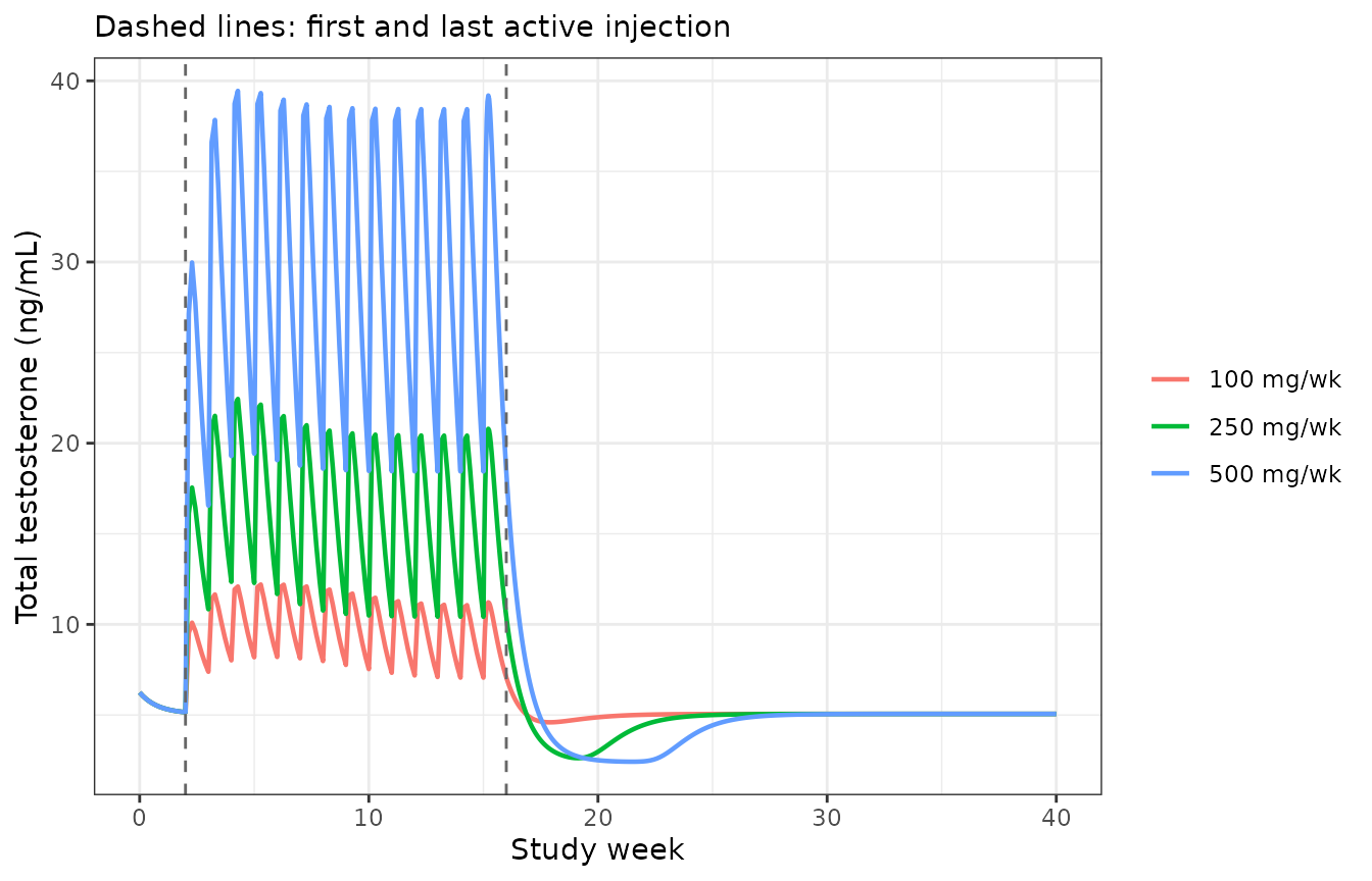
Typical-value total testosterone. Replicates the setting of Bi 2018 Figure 2 (prediction-corrected VPC stratified on dose).
ggplot(sim_typ, aes(week, lh30, colour = treatment)) +
  geom_line(linewidth = 0.8) +
  geom_vline(xintercept = c(2, 16), linetype = "dashed", colour = "grey40") +
  labs(x = "Study week", y = "LH30 (IU/L)", colour = NULL) +
  theme_bw()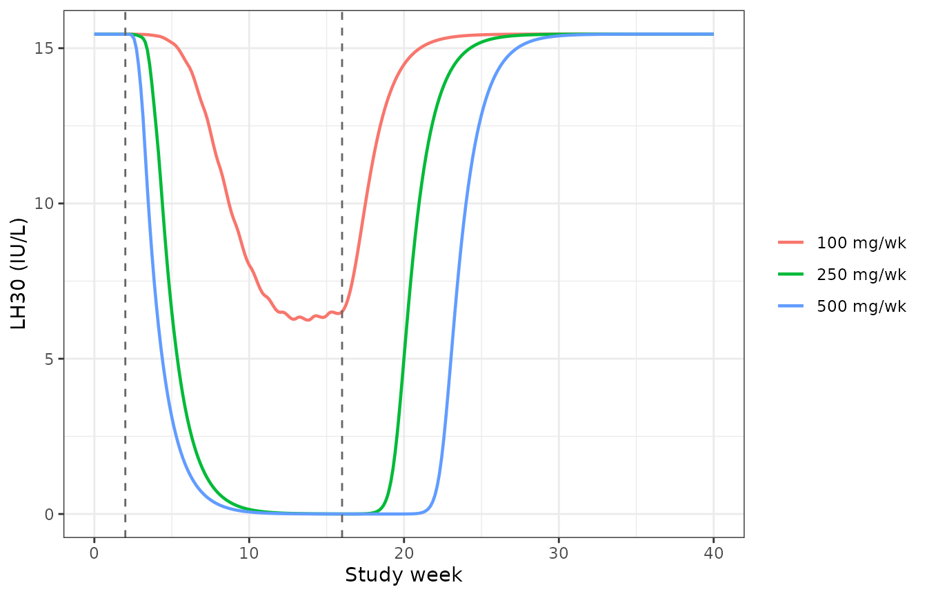
Typical-value LHRH-stimulated LH30. Replicates the left panel of Bi 2018 Figure 3.
Suppression of endogenous testosterone secretion (Figure 4, top panel)
Bi 2018’s Figure 4 plots the suppression of endogenous secretion
against a horizontal dashed line representing “basal endogenous
testosterone secretion independent of LH upregulation” – that is,
b_base. The structural claim is that complete loss of LH
up-regulation drives the secretion rate down to exactly
b_base and no further, and the text states this happened
“during week 9 to week 19 in both the 250 mg and the 500 mg groups”.
b_base <- 6.24
ggplot(sim_typ, aes(week, ksec_te, colour = treatment)) +
  geom_line(linewidth = 0.8) +
  geom_hline(yintercept = b_base, linetype = "dashed", colour = "grey30") +
  labs(x = "Study week", y = "Endogenous secretion (mg/day)", colour = NULL,
       subtitle = "Dashed line: b_base, the LH-independent floor") +
  theme_bw()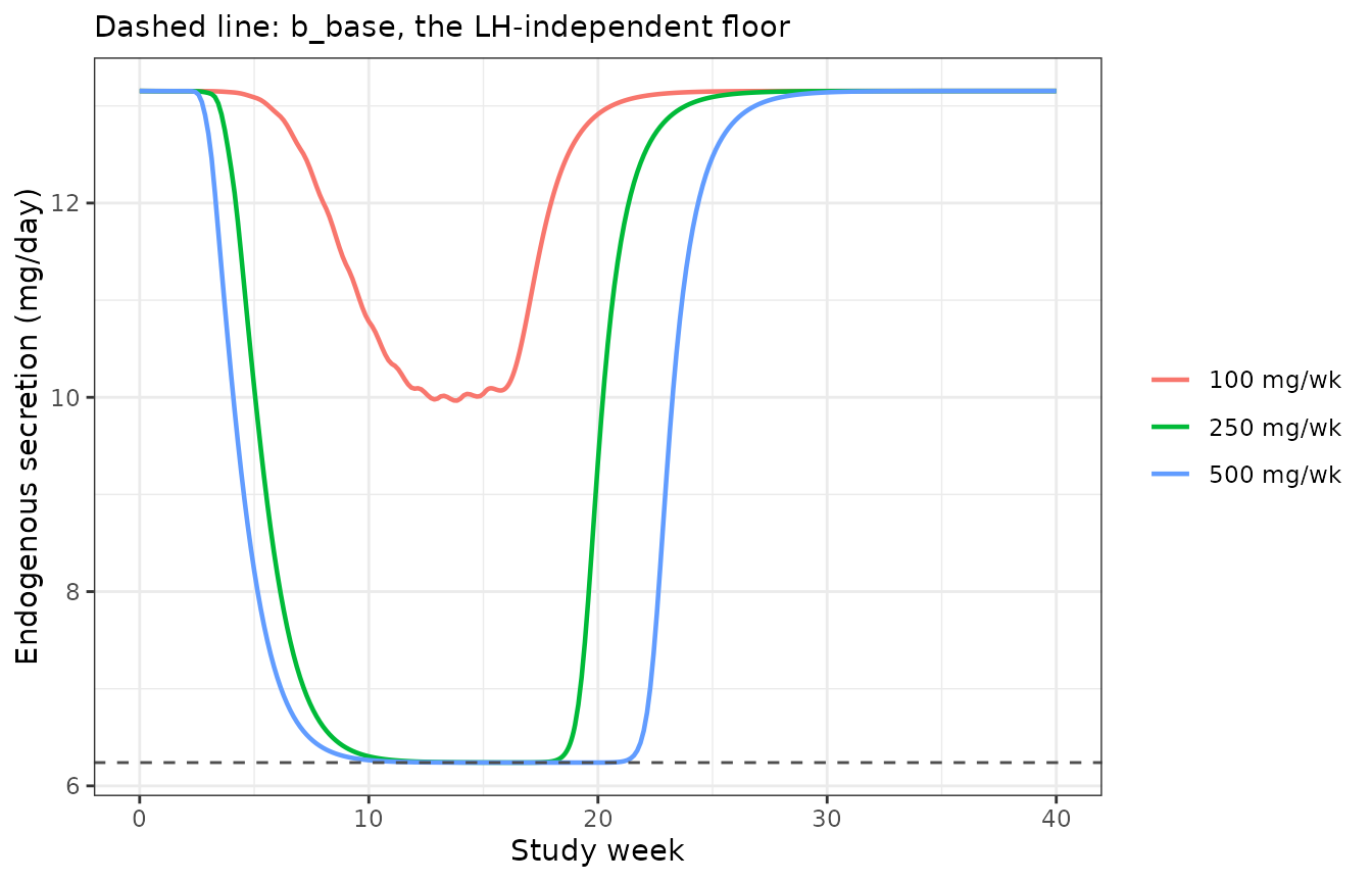
Endogenous testosterone secretion rate. Replicates Bi 2018 Figure 4, top panel.
floors <- sim_typ |>
  dplyr::group_by(treatment) |>
  dplyr::summarise(min_secretion = min(ksec_te), .groups = "drop") |>
  dplyr::mutate(`Reaches b_base` = abs(min_secretion - b_base) < 0.01)
knitr::kable(floors, digits = 4, caption = "Secretion floor by arm.")| treatment | min_secretion | Reaches b_base |
|---|---|---|
| 100 mg/wk | 9.9665 | FALSE |
| 250 mg/wk | 6.2405 | TRUE |
| 500 mg/wk | 6.2400 | TRUE |
# Structural identity: the high-dose arms must land exactly on b_base, and no arm
# may go below it. A sign error or a mis-transcribed b_base breaks both.
stopifnot(
  all(sim_typ$ksec_te >= b_base - 1e-8),
  floors$`Reaches b_base`[floors$treatment == "250 mg/wk"],
  floors$`Reaches b_base`[floors$treatment == "500 mg/wk"]
)
Recovery timing
Bi 2018 reports when suppression of LH synthesis falls back below 10% after the last active injection (study week 15): “in week 10 … in the 500 mg group, compared after week 5 in the 100 mg group and week 6 in the 250 mg group”.
recov <- sim_typ |>
  dplyr::filter(week > 15) |>
  dplyr::group_by(treatment) |>
  dplyr::summarise(
    weeks_after_last_dose = min(week[inh_lh < 0.10]) - 15, .groups = "drop"
  ) |>
  dplyr::mutate(`Bi 2018 Results` = c(5, 6, 10))
knitr::kable(recov, digits = 1,
caption = "Weeks after the last injection until LH-synthesis suppression falls below 10%.")| treatment | weeks_after_last_dose | Bi 2018 Results |
|---|---|---|
| 100 mg/wk | 2.5 | 5 |
| 250 mg/wk | 5.3 | 6 |
| 500 mg/wk | 8.3 | 10 |
# Deterministic typical-value trajectory; the published figures are medians over
# post hoc individuals, so a two-to-three week offset is expected. A bound of 4
# weeks still fails on a mis-transcribed ke0, IC50 or Hill coefficient, each of
# which shifts recovery by many weeks.
stopifnot(all(abs(recov$weeks_after_last_dose - recov$`Bi 2018 Results`) <= 4))
Virtual cohort
A 100-subject-per-arm cohort with the covariate distributions of
Table 1. The Hill coefficient of the LH up-regulation term carries a
proportional random effect in the source control stream
(LAM = TVLAM * (1 + ETA(5))) with a 75.9% coefficient of
variation, so roughly 9% of simulated subjects draw a negative exponent;
this is the authors’ own parameterisation and is discussed in the Errata
below.
n_per_arm <- 100
set.seed(1)
make_cohort <- function(amt, offset) {
  wt <- pmin(pmax(rnorm(n_per_arm, 85, 14), 60.7), 115)
  alb <- pmin(pmax(rnorm(n_per_arm, 45.5, 3.0), 35), 55)
  tibble::tibble(
    id = offset + seq_len(n_per_arm),
    WT_BASE = wt, WT = wt + rnorm(n_per_arm, 2.90, 1.5),
    ALB_BASE = alb, ALB = alb + rnorm(n_per_arm, -2.0, 1.5),
    T4 = pmin(pmax(rnorm(n_per_arm, 7.40, 1.2), 4.5), 12),
    treatment = factor(sprintf("%d mg/wk", amt), levels = sprintf("%d mg/wk", doses))
  )
}
cohort <- dplyr::bind_rows(lapply(seq_along(doses), function(i) {
  make_cohort(doses[i], (i - 1L) * n_per_arm)
}))

vpc_times <- sort(unique(c(seq(0, 280, by = 3.5), seq(105, 133, by = 1))))
events <- cohort |>
  dplyr::select(id, treatment) |>
  tidyr::crossing(time = vpc_times) |>
  dplyr::mutate(evid = 0L, amt = NA_real_, cmt = "central", dvid = 1L)
dose_rows <- cohort |>
  dplyr::select(id, treatment) |>
  tidyr::crossing(time = 14 + 7 * (0:13)) |>
  dplyr::mutate(evid = 1L, cmt = "depot", dvid = NA_integer_) |>
  dplyr::mutate(amt = doses[match(treatment, levels(treatment))])
events <- dplyr::bind_rows(events, dose_rows) |>
  dplyr::left_join(dplyr::select(cohort, -treatment), by = "id") |>
  dplyr::arrange(id, time, dplyr::desc(evid))

sim_cohort <- rxode2::rxSolve(
  uis[[1]], events, returnType = "data.frame", useLinCmt = FALSE,
  keep = c("treatment")
) |>
  dplyr::filter(!is.na(Cc)) |>
  dplyr::mutate(week = time / 7)
cat("cohort rows:", nrow(sim_cohort), " subjects:", dplyr::n_distinct(sim_cohort$id), "\n")
#> cohort rows: 31500  subjects: 300
pctl <- sim_cohort |>
  dplyr::group_by(treatment, week) |>
  dplyr::summarise(
    lo = quantile(ipredSim, 0.025), md = median(ipredSim),
    hi = quantile(ipredSim, 0.975), .groups = "drop"
  )
ggplot(pctl, aes(week)) +
  geom_ribbon(aes(ymin = lo, ymax = hi, fill = treatment), alpha = 0.2) +
  geom_line(aes(y = md, colour = treatment), linewidth = 0.8) +
  labs(x = "Study week", y = "Total testosterone (ng/mL)",
       colour = NULL, fill = NULL) +
  theme_bw()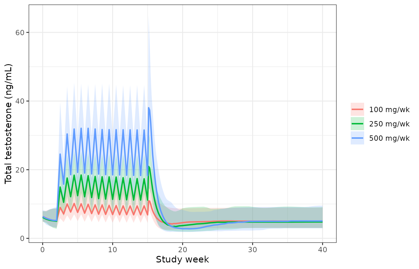
Simulated total testosterone percentiles by arm (2.5th, 50th, 97.5th). Compare Bi 2018 Figure 2.
pctl_lh <- sim_cohort |>
  dplyr::group_by(treatment, week) |>
  dplyr::summarise(
    lo = quantile(lh30, 0.025), md = median(lh30),
    hi = quantile(lh30, 0.975), .groups = "drop"
  )
ggplot(pctl_lh, aes(week)) +
  geom_ribbon(aes(ymin = lo, ymax = hi, fill = treatment), alpha = 0.2) +
  geom_line(aes(y = md, colour = treatment), linewidth = 0.8) +
  labs(x = "Study week", y = "LH30 (IU/L)", colour = NULL, fill = NULL) +
  theme_bw()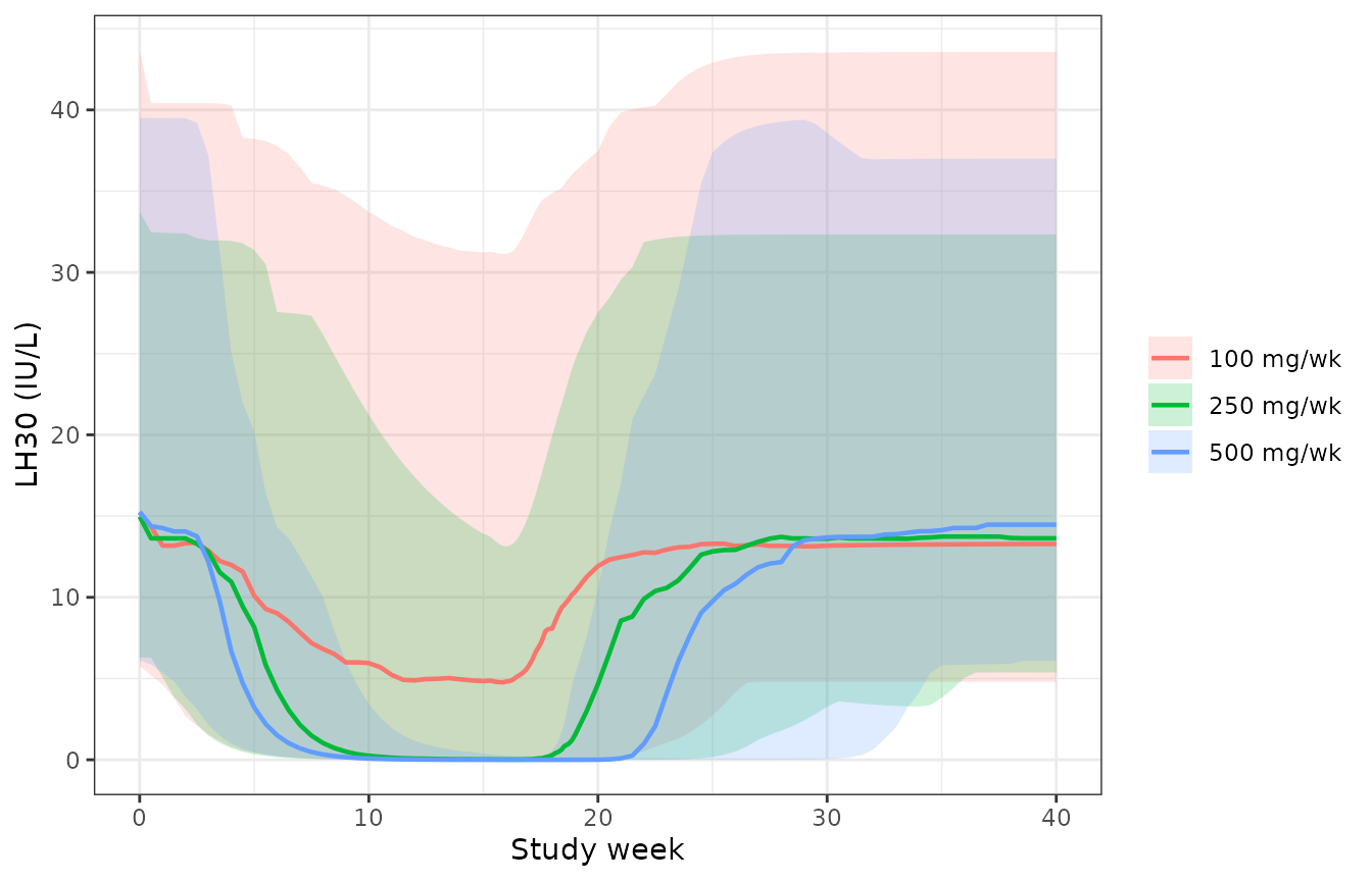
Simulated LH30 percentiles by arm. Compare Bi 2018 Figure 3, left panel.
Bi 2018 reports that LH suppression was severe and consistent in the two high dose arms but variable in the 100 mg arm: “the suppression of LH was more severe in the 250 mg and the 500 mg groups, whereas the suppression is variable in the 100 mg group.”
nadir <- sim_cohort |>
  dplyr::filter(week >= 7, week <= 16) |>
  dplyr::group_by(treatment, id) |>
  dplyr::summarise(max_inh = max(inh_lh), .groups = "drop") |>
  dplyr::group_by(treatment) |>
  dplyr::summarise(
    `Median LH-synthesis suppression` = median(max_inh),
    `5th percentile` = quantile(max_inh, 0.05),
    `Interquartile width` = IQR(max_inh), .groups = "drop"
  )
knitr::kable(nadir, digits = 3,
caption = "Peak LH-synthesis suppression across weeks 7-16, by arm.")| treatment | Median LH-synthesis suppression | 5th percentile | Interquartile width |
|---|---|---|---|
| 100 mg/wk | 0.786 | 0.000 | 0.785 |
| 250 mg/wk | 1.000 | 0.878 | 0.005 |
| 500 mg/wk | 1.000 | 1.000 | 0.000 |
# Cohort-derived, so assert only the ORDERING claim the paper makes, with
# headroom: the two high-dose arms are near-complete and much less dispersed
# than the 100 mg arm.
stopifnot(
  nadir$`Median LH-synthesis suppression`[nadir$treatment == "250 mg/wk"] > 0.9,
  nadir$`Median LH-synthesis suppression`[nadir$treatment == "500 mg/wk"] > 0.9,
  nadir$`Interquartile width`[nadir$treatment == "100 mg/wk"] >
    nadir$`Interquartile width`[nadir$treatment == "500 mg/wk"]
)
Suppression of spermatogenesis
The sperm model consumes CAV, the average total
testosterone concentration over the preceding 18 weeks. Bi 2018 computed
it from the individual post hoc PK predictions; here it is computed from
the typical-value PK simulation above, using the paper’s own rule that
observations earlier than 18 weeks average from the start of the
study.
tau_window <- 18 * 7 # days

cav18 <- function(time, conc) {
  auc <- c(0, cumsum(diff(time) * (head(conc, -1) + tail(conc, -1)) / 2))
  lower <- pmax(0, time - tau_window)
  auc_lower <- approx(time, auc, xout = lower)$y
  width <- pmax(time - lower, .Machine$double.eps)
  out <- (auc - auc_lower) / width
  out[time == 0] <- conc[time == 0] # limit of AUC(t)/t as t -> 0
  out
}

cav_df <- sim_typ |>
  dplyr::group_by(treatment) |>
  dplyr::arrange(time, .by_group = TRUE) |>
  dplyr::mutate(CAV = cav18(time, Cc)) |>
  dplyr::ungroup()
ggplot(cav_df, aes(week, CAV, colour = treatment)) +
  geom_line(linewidth = 0.8) +
  geom_hline(yintercept = 8.68, linetype = "dashed", colour = "grey30") +
  labs(x = "Study week", y = "CAV: 18-week average tT (ng/mL)", colour = NULL,
       subtitle = "Dashed line: Cavg50 = 8.68 ng/mL at 85 kg") +
  theme_bw()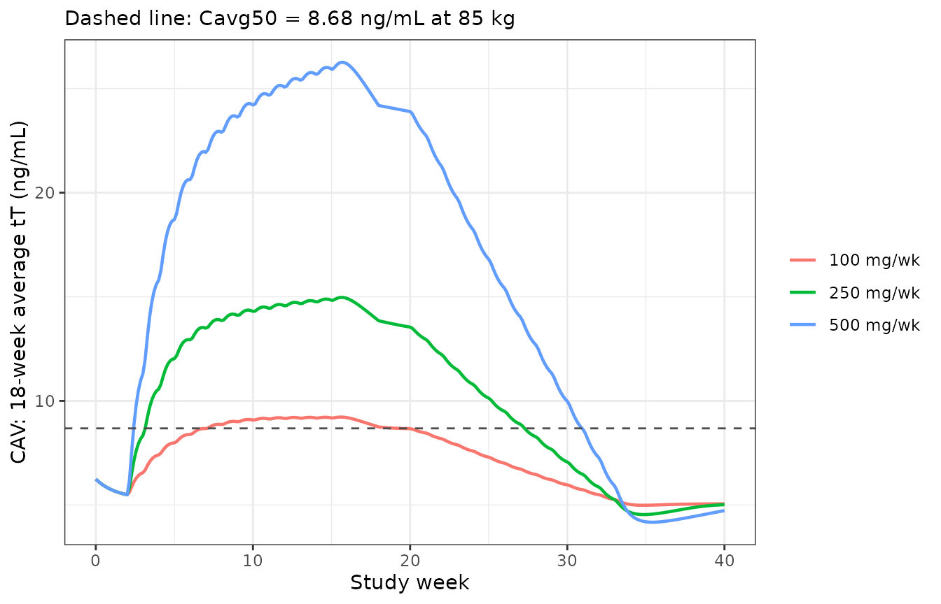
The 18-week rolling average testosterone concentration that drives the spermatogenesis model.
The pre-treatment value of CAV is not zero – the analyte
is endogenous – and the model’s unsuppressed initial condition depends
on that baseline sitting well below Cavg50. That is a
sharper constraint than it looks, because the Hill coefficient is 11.3:
production at baseline must be essentially unsuppressed for
sperm(0) = kin/kout to be a self-consistent initial
condition.
sim_sperm <- dplyr::bind_rows(lapply(levels(cav_df$treatment), function(tr) {
  d <- dplyr::filter(cav_df, treatment == tr)
  ev <- data.frame(id = 1L, time = d$time, evid = 0L, amt = NA_real_,
                   dvid = 1L, CAV = d$CAV, WT_BASE = 85)
  s <- rxode2::rxSolve(sp_typ, ev, returnType = "data.frame", useLinCmt = FALSE)
  s$treatment <- factor(tr, levels = levels(cav_df$treatment))
  s
})) |>
  dplyr::mutate(week = time / 7)
#> ℹ omega/sigma items treated as zero: 'etalkin_sperm', 'etalogitemax_sperm', 'etalic50_sperm', 'etalhill_sperm'
#> ℹ omega/sigma items treated as zero: 'etalkin_sperm', 'etalogitemax_sperm', 'etalic50_sperm', 'etalhill_sperm'
#> ℹ omega/sigma items treated as zero: 'etalkin_sperm', 'etalogitemax_sperm', 'etalic50_sperm', 'etalhill_sperm'

baseline_sperm <- 6.17 / 0.0696
sim_sperm <- dplyr::mutate(
  sim_sperm, suppression = 100 * (1 - sperm / baseline_sperm)
)

# Baseline must be essentially unsuppressed: this is what fixes the weight
# reference at 85 kg rather than the 70 kg printed in the deposited stream.
base_supp <- sim_sperm |>
  dplyr::group_by(treatment) |>
  dplyr::summarise(baseline_suppression = suppression[which.min(time)], .groups = "drop")
knitr::kable(base_supp, digits = 3,
caption = "Suppression of sperm production at time zero (should be near zero).")| treatment | baseline_suppression |
|---|---|
| 100 mg/wk | 0 |
| 250 mg/wk | 0 |
| 500 mg/wk | 0 |
ggplot(sim_sperm, aes(week, sperm, colour = treatment)) +
  geom_line(linewidth = 0.8) +
  geom_vline(xintercept = c(2, 16), linetype = "dashed", colour = "grey40") +
  labs(x = "Study week", y = "Sperm count", colour = NULL) +
  theme_bw()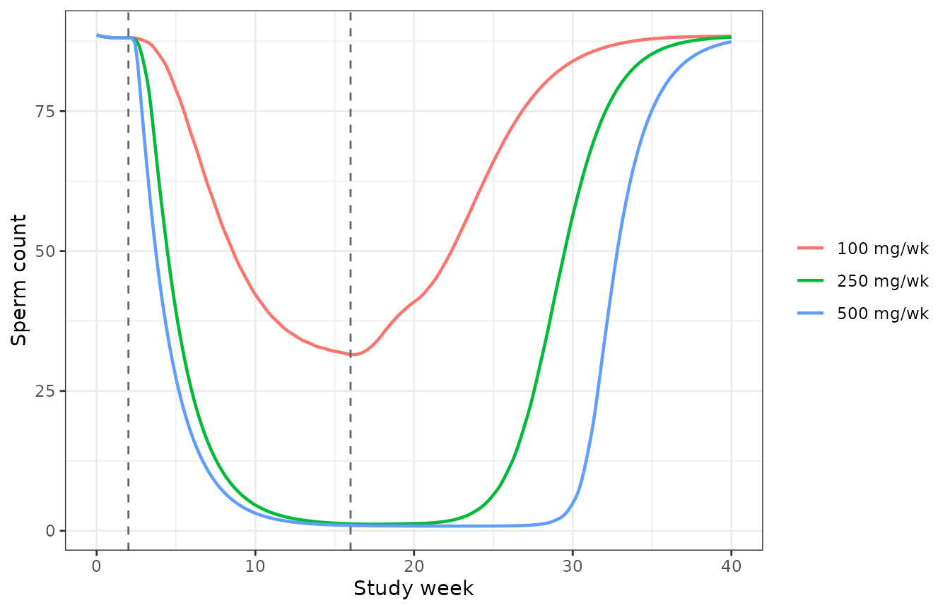
Typical-value sperm count. Replicates Bi 2018 Figure 3 (right panel) and Figure 4 (bottom panel).
at_week <- function(tr, w) {
  d <- dplyr::filter(sim_sperm, treatment == tr)
  approx(d$week, d$suppression, xout = w)$y
}
sperm_claims <- tibble::tribble(
  ~Claim, ~Week, ~Arm, ~`Bi 2018`,
  "Sperm count completely suppressed at the end of dosing", 15, "250 mg/wk", 98.2,
  "Sperm count completely suppressed at the end of dosing", 15, "500 mg/wk", 94.9,
  "Partial recovery by week 28", 28, "100 mg/wk", 26.6,
  "Partial recovery by week 28", 28, "250 mg/wk", 48.4,
  "Partial recovery by week 28", 28, "500 mg/wk", 66.9
) |>
  dplyr::mutate(
    Simulated = mapply(at_week, Arm, Week),
    Deviation = Week == 28
  )
knitr::kable(sperm_claims, digits = 1,
             caption = paste("Suppression of sperm count (%) against Bi 2018's",
                             "post hoc medians. Rows flagged Deviation are not gated;",
"see the Errata."))| Claim | Week | Arm | Bi 2018 | Simulated | Deviation |
|---|---|---|---|---|---|
| Sperm count completely suppressed at the end of dosing | 15 | 250 mg/wk | 98.2 | 98.5 | FALSE |
| Sperm count completely suppressed at the end of dosing | 15 | 500 mg/wk | 94.9 | 98.8 | FALSE |
| Partial recovery by week 28 | 28 | 100 mg/wk | 26.6 | 10.6 | TRUE |
| Partial recovery by week 28 | 28 | 250 mg/wk | 48.4 | 65.8 | TRUE |
| Partial recovery by week 28 | 28 | 500 mg/wk | 66.9 | 98.7 | TRUE |
# The end-of-dosing claim is the one the paper states most confidently and the
# regime where the response is saturated, so it is gated.
stopifnot(
  all(sperm_claims$Simulated[sperm_claims$Week == 15] > 90),
  # Dose ordering of the week-28 recovery is preserved even though the
  # magnitudes are not.
  at_week("500 mg/wk", 28) > at_week("250 mg/wk", 28),
  at_week("250 mg/wk", 28) > at_week("100 mg/wk", 28)
)
At the end of dosing, where the paper’s estimates are precise (“suppression at week 15 and week 21 were precisely estimated”), the model reproduces the published values closely. The week-28 recovery values are systematically higher in the typical-value simulation than in the published post hoc medians. This is expected and the paper anticipates it: recovery “was estimated with wide CIs”, the inter-individual variability on the logit-Emax parameter is 234%, and seven of 29 subjects missed the final collection. A typical-value trajectory is not the median of a cohort that variable, and the paper itself flags the end-of-study estimate as possibly biased.
Assumptions and deviations
Values taken from the supplementary control streams rather than the article
The main article prints the differential equations but not the covariate functional forms, their reference and centring constants, or the residual-error parameterisation. All of these come from the NONMEM control streams in Supplementary Material S6, which were published with the open-access article (PMC5915615). In particular:
- The residual-error scale differs between layers, and the
tables’ labels are wrong in one direction. The PK stream builds
W = SQRT(IPRED*IPRED*THETA(8) + THETA(9))with$SIGMA 1 FIX, so Table 2’ssigma^2 proportional(0.057) andsigma^2 additive(0.261) really are variances and the model file stores their square roots (0.239 and 0.511). The LH and sperm streams instead setW = THETA(6)directly, so Table 3’ssigma^2 additiveentries (0.397 and 0.429) are standard deviations despite the label. Reading either table the other way would misstate the residual magnitude by a factor of roughly two. - Both PD endpoints are fitted on a log(state + 1)
scale (
IPRED = LOG(A(4) + 1)). The+1offset is load-bearing rather than cosmetic, because sperm counts and LH30 both approach zero under complete suppression in the high-dose arms. - The
A_0, TCrow of Table 2 is a concentration, not an amount: the stream computesINT = THETA(10) * EXP(ETA(6))and thenA_0(2) = INT * V. Its value (6.24 ng/mL) coincidentally equalsb_base(6.24 mg/day), which are different quantities with different units, different RSEs and different confidence intervals. - The
$THETAcomment labels in the PK stream are stale and shifted fromTHETA(8)onwards: the entry commented[K1 500mg]is the proportional residual variance,[proportional error]is the additive residual variance, and[additive error]is the baseline concentration. Each was mapped by how the stream uses it, not by its comment, and each maps onto the matching Table 2 row.
The deposited control streams are not uniformly final
The PK and LH streams carry final estimates – 14 of 15 PK
$THETA values and all 6 PK $OMEGA values
reproduce Table 2 exactly, and every LH $THETA and
$OMEGA reproduces Table 3. The sperm-count stream
does not: none of its seven $THETA values matches
Table 3 (for example 0.1 against a final
-1.27, an obvious starting value), and its
$OMEGA entries do not reproduce the published IIV
percentages either. All parameter values in both model files
therefore come from Tables 2 and 3; the streams are used only for model
structure, functional forms and constants.
Two consequences:
-
h Balbumin-V. Table 2 gives the final estimate as -1.55 (bootstrap median -1.84); the PK stream’s$THETA(15)is -1.82851. The model file uses the published -1.55. The parameter has 58.7% RSE, and two other Table 2 parameters (Lambdaand the additive residual) show a comparably large gap between final estimate and bootstrap median, so a final value well away from the bootstrap median is not anomalous here. The albumin effect is one the paper explicitly calls not clinically important. Using -1.83 instead changes the typical volume by under 2% at plausible albumin values. -
The weight reference for
Cavg50. The deposited sperm stream prints(WT/70), but that stream carries starting values throughout. The model file uses 85 kg, on three grounds: it is the typical weight Bi 2018 names in the sentence reporting this very effect; it is the reference used by every other covariate in the paper (85 kg in the PK layer, 84.70 kg in the LH layer); and it is the only choice consistent with the model’s own initial condition. With a 70 kg reference the typicalCavg50at 85 kg falls to 6.78 ng/mL, which – against a baselineCAVnear 6.2 ng/mL and a Hill coefficient of 11.3 – predicts roughly 28% suppression of sperm production in untreated healthy men, contradictingA_0 = KIN/KOUT. The check in the spermatogenesis section above gates exactly this. It also reproduces the paper’s week-28 recovery figures far better (18% versus 78% against a published 26.6% for the 100 mg arm).
Coupling the sequentially-fitted layers
Bi 2018 fitted testosterone PK with LH supplied as a data column and
fitted LH with the PK parameters fixed per subject.
Bi_2018_testosteroneCypionate closes that loop, using the
model’s own lh30 state where the paper used its post hoc
prediction. Two small consequences follow. The stream’s branch
IF (LHORI .EQ. 0) k1 = BASE is replaced by a floor of 1e-8
on the LH driver, which is numerically equivalent and keeps the power
term finite. And the LH stream’s hard-coded initial testosterone
concentration of 6.5 ng/mL (A_0(2) = 6.5*V) is replaced by
the PK model’s own estimated baseline of 6.24 ng/mL, so the two layers
share one baseline instead of two.
The Hill coefficient of the LH up-regulation term can go negative
The PK stream codes LAM = TVLAM * (1 + ETA(5)) – a
proportional, not log-normal, random effect – with $OMEGA
0.576, i.e. a 75.9% CV. Roughly 9% of simulated subjects therefore draw
a negative Hill exponent, which inverts the direction of LH’s effect on
testosterone secretion for those subjects. This is the authors’ own
parameterisation and is reproduced faithfully rather than silently
regularised; the term stays bounded in (0, 1) either way, so it produces
no numerical failure. Users running typical-value simulations
(rxode2::zeroRe()) are unaffected. Note the contrast with
the LH and sperm layers, where the same Hill coefficient carries a
conventional log-normal effect
(LAM = TVLAM * EXP(ETA)).
Covariates
-
T4is total thyroxine, not thyroxine-binding globulin. Bi 2018 Table 1 tabulates thyroxine-binding globulin (group medians 19.5 / 18.5 / 21 ug/mL), but the covariate in the LH control stream isTHYROXINreferenced to 7.40, and the supplementary LH dataset carriesthyroxin = 7.4for its example subject – consistent with total T4 in ug/dL and inconsistent with TBG. The baseline distribution of this covariate is therefore not published, and the virtual cohort above assumes a modest spread around the 7.40 reference. The paper reports that this covariate made no visible difference to simulated LH suppression. - The virtual cohort’s covariate distributions are assumed. Table 1 gives per-arm medians and ranges but no standard deviations and no correlation structure, so normal distributions truncated to the published ranges are used. The weight-change and albumin-change distributions are centred on the model’s own centring constants (+2.90 kg and -0.2 g/dL), which are the cohort medians of those changes, with an assumed spread.
- Serum albumin is held in canonical SI g/L per the nlmixr2lib covariate register, and converted inline to the g/dL scale on which Bi 2018 calibrated its coefficients.
Convention deviations
checkModelConventions() reports one warning on
Bi_2018_testosteroneCypionate_sperm: the single observation
variable logSperm is not a canonical output name. Sperm
count is a genuinely paper-specific endpoint with no canonical
compartment in nlmixr2lib and, as the first paper in the library to
carry it, does not meet the two-paper bar for minting one; the state is
declared through paper_specific_compartments instead. The
remaining message on both models is informational:
units$dosing is mg while units$concentration
is ng/mL, which is correct here because the volumes are expressed in
kilolitres, so mg / kL = ug/L = ng/mL with no conversion
factor.
Not extracted
The sperm-motility model (Supplementary Table S1) and the LH60 and LH120 models are described by Bi 2018 as sensitivity analyses that “had similar parameter estimation and comparable performance”, so they are excluded per nlmixr2lib’s replicate-the-author’s-structure policy, which excludes robustness checks the authors did not report as final.
Session info
sessionInfo()
#> R version 4.6.1 (2026-06-24)
#> Platform: x86_64-pc-linux-gnu
#> Running under: Ubuntu 24.04.5 LTS
#>
#> Matrix products: default
#> BLAS:   /usr/lib/x86_64-linux-gnu/openblas-pthread/libblas.so.3
#> LAPACK: /usr/lib/x86_64-linux-gnu/openblas-pthread/libopenblasp-r0.3.26.so;  LAPACK version 3.12.0
#>
#> locale:
#>  [1] LC_CTYPE=C.UTF-8       LC_NUMERIC=C           LC_TIME=C.UTF-8
#>  [4] LC_COLLATE=C.UTF-8     LC_MONETARY=C.UTF-8    LC_MESSAGES=C.UTF-8
#>  [7] LC_PAPER=C.UTF-8       LC_NAME=C              LC_ADDRESS=C
#> [10] LC_TELEPHONE=C         LC_MEASUREMENT=C.UTF-8 LC_IDENTIFICATION=C
#>
#> time zone: UTC
#> tzcode source: system (glibc)
#>
#> attached base packages:
#> [1] stats     graphics  grDevices utils     datasets  methods   base
#>
#> other attached packages:
#> [1] ggplot2_4.0.3         tidyr_1.3.2           dplyr_1.2.1
#> [4] PKNCA_0.12.1          rxode2_5.1.8          nlmixr2lib_0.3.2.9000
#>
#> loaded via a namespace (and not attached):
#>  [1] gtable_0.3.6        xfun_0.61           bslib_0.12.0
#>  [4] rxode2lincmt_0.1.0  lattice_0.22-9      vctrs_0.7.3
#>  [7] tools_4.6.1         generics_0.1.4      parallel_4.6.1
#> [10] tibble_3.3.1        symengine_0.2.14    pkgconfig_2.0.3
#> [13] data.table_1.18.6.1 checkmate_2.3.4     RColorBrewer_1.1-3
#> [16] S7_0.2.2            desc_1.4.3          lifecycle_1.0.5
#> [19] compiler_4.6.1      farver_2.1.2        textshaping_1.0.5
#> [22] fontawesome_0.5.3   htmltools_0.5.9     sys_3.4.3
#> [25] sass_0.4.10         yaml_2.3.12         pillar_1.11.1
#> [28] pkgdown_2.2.1       crayon_1.5.3        jquerylib_0.1.4
#> [31] whisker_0.4.1       openssl_2.4.2       cachem_1.1.0
#> [34] nlme_3.1-169        tidyselect_1.2.1    digest_0.6.39
#> [37] lotri_1.0.5         purrr_1.2.2         labeling_0.4.3
#> [40] rxode2ll_2.0.18     fastmap_1.2.0       grid_4.6.1
#> [43] cli_3.6.6           dparser_1.3.1-14    magrittr_2.0.5
#> [46] withr_3.0.3         scales_1.4.0        backports_1.5.1
#> [49] rmarkdown_2.32      otel_0.2.0          askpass_1.2.1
#> [52] ragg_1.5.2          memoise_2.0.1       evaluate_1.0.5
#> [55] knitr_1.52          rex_1.2.2           PreciseSums_0.7
#> [58] rlang_1.3.0         downlit_0.4.5       Rcpp_1.1.2
#> [61] glue_1.8.1          xml2_1.6.0          jsonlite_2.0.0
#> [64] R6_2.6.1            systemfonts_1.3.2   fs_2.1.0