Vericiguat (Ruehs 2021)
Source:vignettes/articles/Ruehs_2021_vericiguat.Rmd
Ruehs_2021_vericiguat.RmdModel and source
Ruehs 2021 reports two models from the phase II SOCRATES-REDUCED study, and both are packaged:
Ruehs_2021_vericiguat– the final covariate population PK model (Table 2).Ruehs_2021_vericiguat_ntprobnp– the NT-proBNP turnover PK/PD model (Table 3, Eqs. 4-6), driven by the paper’s PK base model (Table 1). The paper states that “the PK base model was used to generate PK/PD simulations”; the Figure 7 replication below confirms it.Citation: Ruehs H, Klein D, Frei M, Grevel J, Austin R, Becker C, Roessig L, Pieske B, Garmann D, Meyer M. Population Pharmacokinetics and Pharmacodynamics of Vericiguat in Patients with Heart Failure and Reduced Ejection Fraction. Clin Pharmacokinet. 2021;60(11):1407-1421. doi:10.1007/s40262-021-01024-y
Description (PK): One-compartment population PK model with first-order absorption for oral vericiguat (a soluble guanylate cyclase stimulator) in adults with worsening chronic heart failure and left ventricular ejection fraction < 45% from the phase II SOCRATES-REDUCED study (final covariate model). Apparent clearance is scaled by body weight (fixed exponent 0.75), age, total bilirubin and creatinine clearance standardized to 70 kg; apparent volume by body weight (fixed exponent 1) and sex; and the absorption rate constant by body weight and serum albumin. Relative bioavailability falls stepwise with the administered dose level (1.08, 1, 0.867, 0.793 at 1.25, 2.5, 5, 10 mg). Residual error is combined proportional plus additive.
Description (PK/PD): PK/PD turnover model for the effect of oral vericiguat on plasma NT-proBNP in adults with worsening chronic heart failure and left ventricular ejection fraction < 45% (phase II SOCRATES-REDUCED). The PK layer is the paper’s PK base model (one compartment, first-order absorption, correlated IIV on CL/F and V/F, no covariates), which the authors used to generate the exposure for the PK/PD analysis. NT-proBNP follows a turnover model whose zero-order production rises with the log of the individual baseline and is inhibited linearly by the 24-h vericiguat AUC, and whose first-order elimination is itself inhibited by NT-proBNP (Emax fixed at 0.95). Without drug the model is not at equilibrium at baseline, so NT-proBNP drifts downward on standard of care alone (the placebo arm). Residual error is additive on the log scale.
Article (open access): https://doi.org/10.1007/s40262-021-01024-y
Supplement (ESM 1: sampling scheme, model-development run records, stepwise covariate table, steady-state exposure statistics by dose): available from the article page.
Vericiguat is an oral soluble guanylate cyclase stimulator approved for chronic heart failure with reduced ejection fraction after a worsening event. SOCRATES-REDUCED randomised patients to placebo or to vericiguat once daily with target doses of 1.25, 2.5, 5 or 10 mg for 12 weeks; the 5 and 10 mg arms started at 2.5 mg and were up-titrated at weeks 2 and 4 depending on blood pressure and tolerability.
Population
The PK analysis used 454 of the 456 randomised patients; 363 received vericiguat and contributed 3376 eligible plasma samples (Ruehs 2021 Section 3.1, Fig. 1). The NT-proBNP analysis used 2347 samples from 432 patients in all five arms. All patients had worsening chronic heart failure with left ventricular ejection fraction < 45% on guideline-directed standard of care. The paper prints no demographics table; the covariate medians it normalises to are age 68 years, body weight 70 kg, bilirubin 0.6 mg/dL, creatinine clearance standardized to 70 kg of 100 mL/min, and albumin 4.0 g/dL (Table 2 footnote). Baseline NT-proBNP ranged from 94.1 to 69,720 pg/mL with quartile boundaries 1559, 3000 and 6246 pg/mL (Section 2.6).
The same information is available programmatically via
readModelDb("Ruehs_2021_vericiguat")()$population and
readModelDb("Ruehs_2021_vericiguat_ntprobnp")()$population.
Source trace
Every ini() value carries an in-file comment naming its
source. The table collects them.
| Model | Parameter / equation | Value | Source location |
|---|---|---|---|
| PK final | lka |
log(1.29) 1/h | Table 2 |
| PK final | lcl |
log(1.24) L/h | Table 2 |
| PK final | lvc |
log(34.3) L | Table 2 (footnote equation prints 3.43, a typo) |
| PK final | e_age_cl |
-0.418 | Table 2, theta CL,age; reference 68 years |
| PK final | e_wt_cl |
0.75 (fixed) | Table 2 footnote b; Eq. 2; reference 70 kg |
| PK final | e_crcl_cl |
0.164 | Table 2; reference 100 mL/min |
| PK final | e_tbili_cl |
-0.072 | Table 2 (footnote equation prints -0.075); reference 0.6 mg/dL |
| PK final | e_wt_vc |
1 (fixed) | Table 2 footnote b; Eq. 3 |
| PK final | e_sexf_vc |
0.850 | Table 2, theta V,sex (female / male) |
| PK final | e_wt_ka |
1.28 | Table 2; reference 70 kg |
| PK final | e_alb_ka |
2.37 | Table 2; reference 4.0 g/dL |
| PK final |
e_dose_1p25mg_fdepot, e_dose_5mg_fdepot,
e_dose_10mg_fdepot
|
1.08, 0.867, 0.793 | Table 2 and footnote (F = 1 at 2.5 mg) |
| PK final |
etalka, etalcl, etalvc
|
0.867, 0.061, 0.043 | ESM Table 3 run 10 (reproduce the Table 2 CVs 117%, 25.1%, 21.0%) |
| PK final |
propSd, addSd
|
0.257, 7.27 ug/L | Table 2 |
| PK/PD |
lka, lcl, lvc
|
log(1.5), log(1.3), log(38.9) | Table 1 (PK base model) |
| PK/PD | etalcl + etalvc |
0.13802, 0.07201, 0.076677 | Table 1: CV 38.47%, 28.23%, correlation 0.70; omega^2 = log(CV^2 + 1) |
| PK/PD | etalka |
0.72304 | Table 1: CV 102.99% |
| PK/PD |
propSd, addSd
|
0.2602, 7.81 ug/L | Table 1 |
| PK/PD | lkin |
log(77.4) pg/mL/day | Table 3, TVkin |
| PK/PD | lrbase |
log(3140) pg/mL | Table 3, [NT-proBNP]baseline |
| PK/PD | e_rbase_kin |
0.347 | Table 3, theta kin,NT-proBNP; Eq. 6 |
| PK/PD | lkout_max |
log(0.157) 1/day | Table 3 |
| PK/PD | emax |
0.95 (fixed) | Table 3 |
| PK/PD | lec50 |
log(439) pg/mL | Table 3 |
| PK/PD | e_auc_kin |
0.0176 L/h/mg | Table 3, ATRT; Eq. 6 |
| PK/PD |
etalkin, etalrbase
|
0.163, 0.953 | Table 3 |
| PK/PD | expSd_ntprobnp |
sqrt(0.145) = 0.38079 | Table 3, additive error variance on log NT-proBNP |
| PK/PD | d/dt(ntprobnp) = kin - kout * ntprobnp |
– | Eq. 4 |
| PK/PD | kout = kout_max * (1 - Emax * N / (EC50 + N)) |
– | Eq. 5 |
| PK/PD | kin = TVkin * (1 + theta * (ln(BL) - 8.03)) * (1 - ATRT * AUC) |
– | Eq. 6 |
| PK/PD |
auc24 = 24 * C(t) (mg*h/L) |
– | Section 2.4 (24-h AUC updated every 24 h); see Assumptions |
# rxode2 warns when a multi-subject solve has no omega; every solve below uses
# zeroRe() with the etas supplied as data columns (drawn with base R), so that
# warning is expected and is the only one muffled.
solve_quiet <- function(model, events) {
  withCallingHandlers(
    rxode2::rxSolve(model, events = events, returnType = "data.frame"),
    warning = function(w) {
      if (grepl("omega", conditionMessage(w))) invokeRestart("muffleWarning")
    }
  )
}

# Dose on study day d (0-based) for each SOCRATES-REDUCED arm: the 5 and 10 mg
# arms started at 2.5 mg and were up-titrated at weeks 2 and 4 (Section 2.1).
arm_dose <- function(arm, day) {
  switch(arm,
    "Placebo" = rep(0, length(day)),
    "1.25 mg" = rep(1.25, length(day)),
    "2.5 mg" = rep(2.5, length(day)),
    "5 mg" = ifelse(day < 14, 2.5, 5),
    "10 mg" = ifelse(day < 14, 2.5, ifelse(day < 28, 5, 10))
  )
}

mod_pk <- rxode2::rxode2(readModelDb("Ruehs_2021_vericiguat"))
#> ℹ parameter labels from comments will be replaced by 'label()'
mod_pd <- rxode2::rxode2(readModelDb("Ruehs_2021_vericiguat_ntprobnp"))
#> ℹ parameter labels from comments will be replaced by 'label()'
Final PK model (Table 2)
Typical patient at steady state
Once-daily dosing for 21 days in the reference patient (male, 70 kg,
68 years, bilirubin 0.6 mg/dL = 10.26 umol/L, standardized creatinine
clearance 100 mL/min, albumin 4.0 g/dL = 40 g/L). The steady-state AUC
over a dosing interval must equal F * Dose / (CL/F)
exactly, which checks the dose-level bioavailability step function; it
is then compared with the geometric-mean individual AUC(tau,ss) of ESM
Table 4.
doses <- c(1.25, 2.5, 5, 10)
f_rel <- c(1.08, 1, 0.867, 0.793)
last_dose <- 20 * 24

ev_typ <- lapply(seq_along(doses), function(i) {
  obs_t <- sort(unique(c(last_dose + seq(0, 24, by = 0.25), 0)))
  bind_rows(
    tibble(id = i, time = (0:20) * 24, evid = 1, amt = doses[i], cmt = "depot"),
    tibble(id = i, time = obs_t, evid = 0, amt = 0, cmt = "central")
  ) |>
    mutate(DOSE = doses[i], WT = 70, AGE = 68, TBILI = 0.6 * 17.1, CRCL = 100, ALB = 40, SEXF = 0)
}) |>
  bind_rows() |>
  arrange(id, time, desc(evid)) |>
  relocate(id, time, evid, amt, cmt)

sim_typ <- solve_quiet(rxode2::zeroRe(mod_pk), ev_typ) |>
  mutate(dose_mg = doses[id])
#> ℹ omega/sigma items treated as zero: 'etalka', 'etalcl', 'etalvc'

conc_typ <- PKNCA::PKNCAconc(
  sim_typ |> select(id, time, Cc, dose_mg),
  Cc ~ time | dose_mg + id,
  concu = "ug/L", timeu = "h"
)
dose_typ <- PKNCA::PKNCAdose(
  ev_typ |> filter(evid == 1) |> mutate(dose_mg = doses[id]) |> select(id, time, amt, dose_mg),
  amt ~ time | dose_mg + id,
  doseu = "mg"
)
nca_typ <- PKNCA::pk.nca(PKNCA::PKNCAdata(
  conc_typ, dose_typ,
  intervals = data.frame(start = last_dose, end = last_dose + 24, auclast = TRUE)
))

typ_tbl <- as.data.frame(nca_typ$result) |>
  filter(PPTESTCD == "auclast") |>
  select(dose_mg, auc_sim = PPORRES) |>
  mutate(
    auc_closed = 1000 * f_rel[match(dose_mg, doses)] * dose_mg / 1.24,
    esm_geomean = c(1069.344, 2053.981, 3513.932, 6247.014)[match(dose_mg, doses)],
    pct_vs_esm = 100 * (auc_sim / esm_geomean - 1)
  )

typ_tbl |>
  mutate(dose_mg = format(dose_mg)) |>
  rename(
    "Dose (mg)" = dose_mg,
    "Simulated AUCtau,ss (ug*h/L)" = auc_sim,
    "F x Dose / (CL/F) (ug*h/L)" = auc_closed,
    "ESM Table 4 geometric mean (ug*h/L)" = esm_geomean,
    "% difference vs ESM" = pct_vs_esm
  ) |>
knitr::kable(digits = 1, caption = "Typical-patient steady-state AUC over a 24-h dosing interval.")| Dose (mg) | Simulated AUCtau,ss (ug*h/L) | F x Dose / (CL/F) (ug*h/L) | ESM Table 4 geometric mean (ug*h/L) | % difference vs ESM |
|---|---|---|---|---|
| 1.25 | 1088.4 | 1088.7 | 1069.3 | 1.8 |
| 2.50 | 2015.6 | 2016.1 | 2054.0 | -1.9 |
| 5.00 | 3495.1 | 3496.0 | 3513.9 | -0.5 |
| 10.00 | 6393.6 | 6395.2 | 6247.0 | 2.3 |
stopifnot(
  # Structural identity (same parameters on both sides): only the trapezoid
  # error of the 15-min grid separates them.
  all(abs(typ_tbl$auc_sim / typ_tbl$auc_closed - 1) < 0.002),
  # The typical patient sits within 3% of the individual geometric means at
  # every dose level (-1.8% to +2.4% observed); a mis-transcribed CL/F or F
  # step moves at least one dose level by 8% or more.
  all(abs(typ_tbl$pct_vs_esm) < 5)
)
Virtual cohort and steady-state NCA
The paper does not print covariate distributions, so the virtual cohort centres every covariate on the median printed in the Table 2 footnote with an assumed spread (see Assumptions). 200 patients per fixed-dose arm take vericiguat once daily for 21 days; the cohort and the between-subject random effects are drawn with base R, so the result does not depend on the rxode2 build or thread count.
set.seed(20210604)
n_arm <- 200

draw_trunc <- function(n, rfun, lo, hi) {
  x <- rfun(n)
  while (any(bad <- x < lo | x > hi)) x[bad] <- rfun(sum(bad))
  x
}

pk_patients <- tibble(
  pid = seq_len(n_arm),
  WT = draw_trunc(n_arm, function(n) rlnorm(n, log(70), 0.2), 40, 150),
  AGE = draw_trunc(n_arm, function(n) rnorm(n, 68, 11), 23, 95),
  SEXF = rbinom(n_arm, 1, 0.25),
  TBILI = 17.1 * rlnorm(n_arm, log(0.6), 0.5),
  CRCL = draw_trunc(n_arm, function(n) rlnorm(n, log(100), 0.3), 20, 250),
  ALB = 10 * draw_trunc(n_arm, function(n) rnorm(n, 4.0, 0.4), 2.5, 5.5),
  etalka = rnorm(n_arm, 0, sqrt(0.867)),
  etalcl = rnorm(n_arm, 0, sqrt(0.061)),
  etalvc = rnorm(n_arm, 0, sqrt(0.043))
)

# The same 200 patients receive each dose level (disjoint ids per arm), so
# between-arm differences reflect dose and bioavailability, not sampling.
ev_pk <- lapply(seq_along(doses), function(i) {
  pts <- pk_patients |> mutate(id = (i - 1) * 1000 + pid, dose_mg = doses[i])
  obs_t <- c(0, last_dose + c(0, 0.5, 1, 1.5, 2, 2.5, 3, 4, 5, 6, 8, 12, 16, 20, 24))
  bind_rows(
    tidyr::crossing(pts, time = (0:20) * 24) |> mutate(evid = 1, amt = dose_mg, cmt = "depot"),
    tidyr::crossing(pts, time = obs_t) |> mutate(evid = 0, amt = 0, cmt = "central")
  )
}) |>
  bind_rows() |>
  mutate(DOSE = dose_mg) |>
  arrange(id, time, desc(evid)) |>
  relocate(id, time, evid, amt, cmt)
stopifnot(!anyDuplicated(unique(ev_pk[, c("id", "time", "evid")])))

sim_pk <- solve_quiet(rxode2::zeroRe(mod_pk), ev_pk) |>
  mutate(dose_mg = doses[(id %/% 1000) + 1])
#> ℹ omega/sigma items treated as zero: 'etalka', 'etalcl', 'etalvc'

sim_nca <- sim_pk |>
  filter(!is.na(Cc)) |>
  select(id, time, Cc, dose_mg)
sim_nca <- bind_rows(
  sim_nca,
  sim_nca |> distinct(id, dose_mg) |> mutate(time = 0, Cc = 0)
) |>
  distinct(id, dose_mg, time, .keep_all = TRUE) |>
  arrange(id, dose_mg, time)

conc_obj <- PKNCA::PKNCAconc(sim_nca, Cc ~ time | dose_mg + id, concu = "ug/L", timeu = "h")
dose_obj <- PKNCA::PKNCAdose(
  ev_pk |> filter(evid == 1) |> select(id, time, amt, dose_mg),
  amt ~ time | dose_mg + id,
  doseu = "mg"
)
nca_pk <- PKNCA::pk.nca(PKNCA::PKNCAdata(
  conc_obj, dose_obj,
  intervals = data.frame(
    start = last_dose, end = last_dose + 24,
    cmax = TRUE, auclast = TRUE, cmin = TRUE
  )
))
ESM Table 4 reports descriptive statistics of the individual steady-state exposures of the study patients; its medians are compared with the medians of the virtual cohort.
published_pk <- tibble::tribble(
  ~dose_mg, ~auclast, ~cmax, ~cmin,
  1.25, 1000.559, 55.732, 27.838,
  2.5, 1998.008, 114.708, 55.82,
  5, 3668.427, 205.521, 105.169,
  10, 6327.505, 348.508, 176.512
)

cmp_pk <- nlmixr2lib::ncaComparisonTable(
  simulated = nca_pk,
  reference = published_pk,
  by = "dose_mg",
  units = c(auclast = "ug*h/L", cmax = "ug/L", cmin = "ug/L"),
  tolerance_pct = 20
)
knitr::kable(
  cmp_pk,
  caption = paste(
    "Median steady-state exposure, virtual cohort vs ESM Table 4 medians",
    "(the ESM Ctrough,ss is compared with the simulated interval minimum,",
    "which for once-daily oral dosing at steady state is the pre-dose trough).",
    "* differs from the reference by more than 20%."
  )
)| NCA parameter | dose_mg | Reference | Simulated | % diff |
|---|---|---|---|---|
| Cmax (ug/L) | 1.25 | 55.7 | 66 | +18.4% |
| Cmax (ug/L) | 2.50 | 115 | 122 | +6.6% |
| Cmax (ug/L) | 5.00 | 206 | 212 | +3.1% |
| Cmax (ug/L) | 10.00 | 349 | 388 | +11.3% |
| Cmin (ug/L) | 1.25 | 27.8 | 29.5 | +5.9% |
| Cmin (ug/L) | 2.50 | 55.8 | 54.6 | -2.2% |
| Cmin (ug/L) | 5.00 | 105 | 94.6 | -10.0% |
| Cmin (ug/L) | 10.00 | 177 | 173 | -1.9% |
| AUClast (ug*h/L) | 1.25 | 1000 | 1130 | +13.3% |
| AUClast (ug*h/L) | 2.50 | 2000 | 2100 | +5.1% |
| AUClast (ug*h/L) | 5.00 | 3670 | 3640 | -0.8% |
| AUClast (ug*h/L) | 10.00 | 6330 | 6660 | +5.2% |
pk_med <- as.data.frame(nca_pk$result) |>
  group_by(dose_mg, PPTESTCD) |>
  summarise(sim = median(PPORRES), .groups = "drop") |>
  inner_join(
    published_pk |> pivot_longer(-dose_mg, names_to = "PPTESTCD", values_to = "ref"),
    by = c("dose_mg", "PPTESTCD")
  ) |>
  mutate(pct = 100 * (sim / ref - 1))

auc_pct <- pk_med$pct[pk_med$PPTESTCD == "auclast"]
cmax_pct <- pk_med$pct[pk_med$PPTESTCD == "cmax"]
stopifnot(
  # The cohort covariates are assumptions (the paper prints none) and the
  # published medians come from 40-71 patients per arm, so these bounds are
  # wider than the typical-patient check above. The cohort and the random
  # effects are drawn with base R and the solve is deterministic, so the
  # values below (AUC -1% to +13%, Cmax +3% to +18%) do not move across
  # machines.
  abs(median(auc_pct)) < 10,
  all(abs(auc_pct) < 15),
  all(abs(cmax_pct) < 25)
)
sim_pk |>
  filter(time >= last_dose) |>
  mutate(tad = time - last_dose, dose = factor(paste(dose_mg, "mg"), paste(doses, "mg"))) |>
  group_by(dose, tad) |>
  summarise(
    q05 = quantile(Cc, 0.05), q50 = median(Cc), q95 = quantile(Cc, 0.95),
    .groups = "drop"
  ) |>
  ggplot(aes(tad, q50, colour = dose, fill = dose)) +
  geom_ribbon(aes(ymin = q05, ymax = q95), alpha = 0.15, colour = NA) +
  geom_line() +
  scale_y_log10() +
  labs(
    x = "Time after dose at steady state (h)", y = "Vericiguat Cc (ug/L)",
    colour = "Dose", fill = "Dose",
    caption = "Median and 90% interval of the virtual cohort (individual predictions)."
  )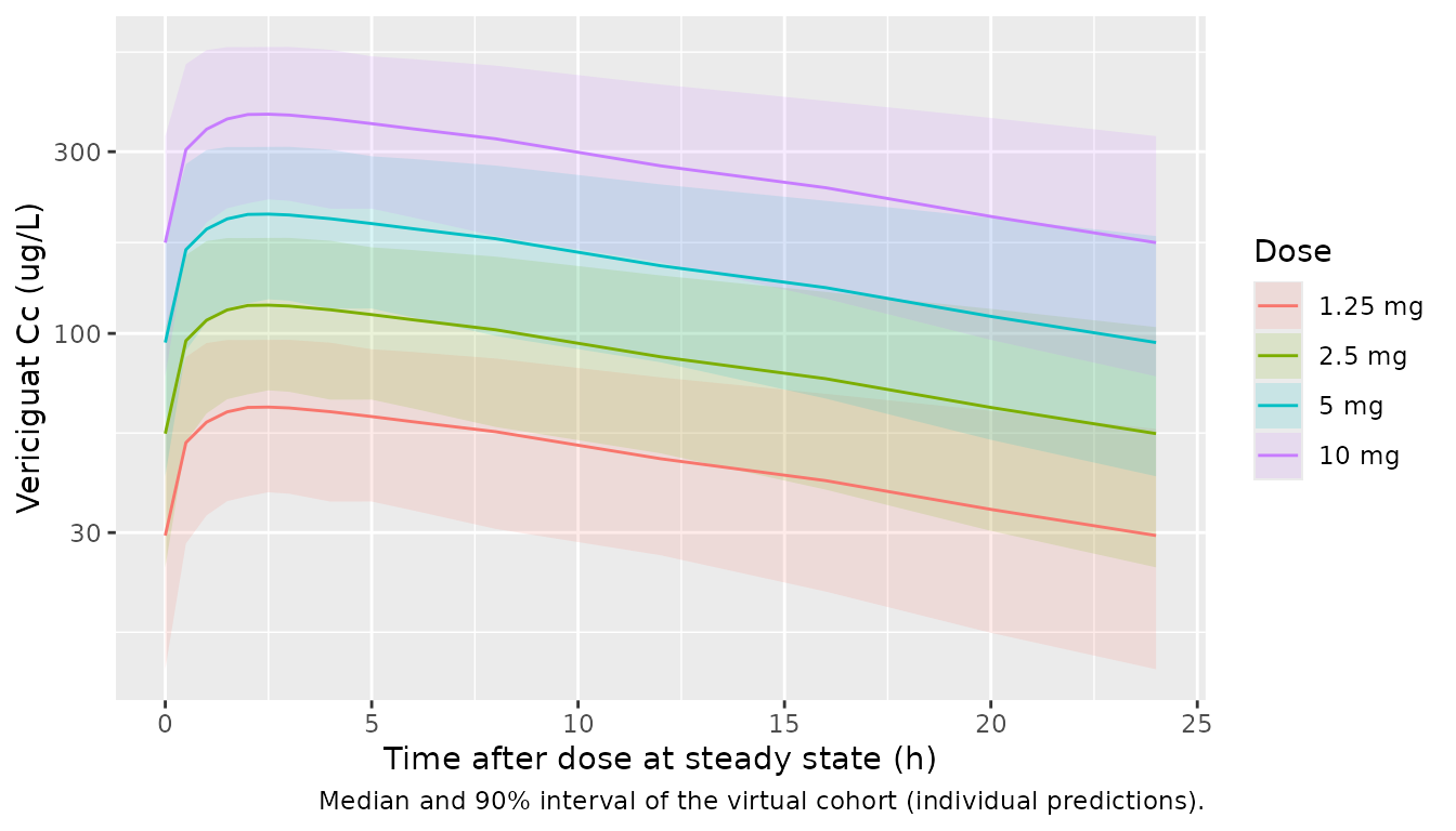
The dose-level bioavailability makes exposure less than dose-proportional: the typical dose-normalised AUC at 10 mg is 73% of that at 1.25 mg, matching the ratio of the ESM Table 4 geometric means (73%).
NT-proBNP PK/PD model (Table 3)
Typical-patient time courses (Figure 7)
Figure 7 simulates typical patients with six baseline NT-proBNP
values under standard of care alone (placebo) and with vericiguat
titrated to 10 mg for 12 weeks, followed by 8 weeks off treatment. The
individual baseline enters both the initial condition and the production
rate (Eq. 6), so each baseline is set through lrbase on the
zero-random-effect model.
baselines <- c(250, 500, 1000, 3000, 5000, 10000)
days_obs <- 0:140

pd_events <- function(arm) {
  dose_days <- if (arm == "Placebo") integer(0) else 0:83
  bind_rows(
    tibble(time = dose_days * 24, evid = 1, amt = arm_dose(arm, dose_days), cmt = "depot"),
    tibble(time = days_obs * 24, evid = 0, amt = 0, cmt = "ntprobnp")
  ) |>
    mutate(id = 1L) |>
    arrange(time, desc(evid)) |>
    relocate(id, time, evid, amt, cmt)
}

# The baseline is set through the baseline random effect, supplied as a data
# column to the zero-random-effect model: etalrbase = log(baseline / 3140).
run_typical <- function(model, bl, arm, ev = pd_events(arm)) {
  ev <- ev |> mutate(etalrbase = log(bl / 3140))
  solve_quiet(rxode2::zeroRe(model), ev) |>
    filter(!is.na(ntprobnp)) |>
    transmute(day = time / 24, ntprobnp, baseline = bl, arm = arm)
}

fig7 <- bind_rows(lapply(baselines, function(b) {
  bind_rows(run_typical(mod_pd, b, "10 mg"), run_typical(mod_pd, b, "Placebo"))
}))
#> ℹ omega/sigma items treated as zero: 'etalcl', 'etalvc', 'etalka', 'etalkin', 'etalrbase'
#> ℹ omega/sigma items treated as zero: 'etalcl', 'etalvc', 'etalka', 'etalkin', 'etalrbase'
#> ℹ omega/sigma items treated as zero: 'etalcl', 'etalvc', 'etalka', 'etalkin', 'etalrbase'
#> ℹ omega/sigma items treated as zero: 'etalcl', 'etalvc', 'etalka', 'etalkin', 'etalrbase'
#> ℹ omega/sigma items treated as zero: 'etalcl', 'etalvc', 'etalka', 'etalkin', 'etalrbase'
#> ℹ omega/sigma items treated as zero: 'etalcl', 'etalvc', 'etalka', 'etalkin', 'etalrbase'
#> ℹ omega/sigma items treated as zero: 'etalcl', 'etalvc', 'etalka', 'etalkin', 'etalrbase'
#> ℹ omega/sigma items treated as zero: 'etalcl', 'etalvc', 'etalka', 'etalkin', 'etalrbase'
#> ℹ omega/sigma items treated as zero: 'etalcl', 'etalvc', 'etalka', 'etalkin', 'etalrbase'
#> ℹ omega/sigma items treated as zero: 'etalcl', 'etalvc', 'etalka', 'etalkin', 'etalrbase'
#> ℹ omega/sigma items treated as zero: 'etalcl', 'etalvc', 'etalka', 'etalkin', 'etalrbase'
#> ℹ omega/sigma items treated as zero: 'etalcl', 'etalvc', 'etalka', 'etalkin', 'etalrbase'
fig7 |>
  mutate(baseline = factor(baseline), arm = ifelse(arm == "Placebo", "Placebo", "Vericiguat")) |>
  ggplot(aes(day / 7, ntprobnp, colour = baseline, linetype = arm)) +
  geom_line() +
  labs(
    x = "Time (weeks)", y = "NT-proBNP (pg/mL)", colour = "Baseline (pg/mL)",
    linetype = "Treatment",
    caption = "Replicates Figure 7a of Ruehs 2021."
  )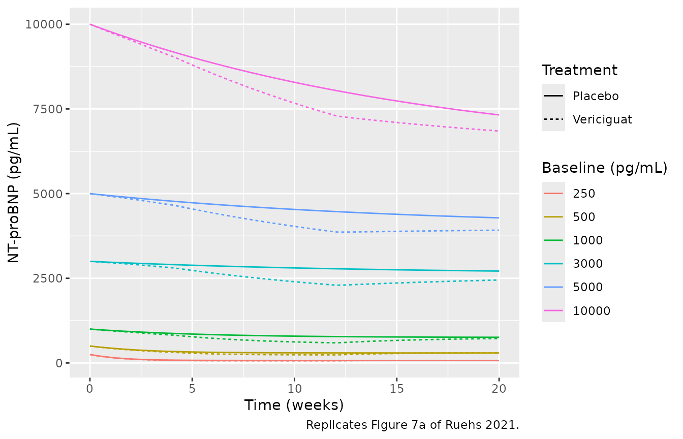
fig7_diff <- fig7 |>
  select(day, baseline, arm, ntprobnp) |>
  pivot_wider(names_from = arm, values_from = ntprobnp) |>
  mutate(diff = `10 mg` - Placebo)

fig7_diff |>
  ggplot(aes(day / 7, diff, colour = factor(baseline))) +
  geom_line() +
  labs(
    x = "Time (weeks)", y = "Placebo-adjusted change in NT-proBNP (pg/mL)",
    colour = "Baseline (pg/mL)",
    caption = "Replicates Figure 7b of Ruehs 2021."
  )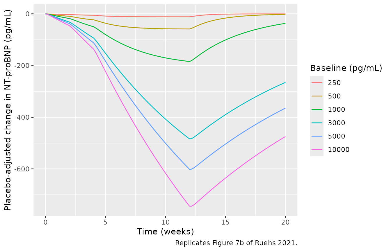
Section 4.3 of the paper prints the week-12 values of Figure 7b: absolute placebo-adjusted decreases of 11, 58, 183, 478, 593 and 734 pg/mL (5%, 12%, 18%, 16%, 12% and 7% of baseline) for baselines of 250 to 10,000 pg/mL.
published_7b <- tibble(
  baseline = baselines,
  paper_diff = c(11, 58, 183, 478, 593, 734),
  paper_pct = c(5, 12, 18, 16, 12, 7)
)

fig7_wk12 <- fig7_diff |>
  filter(day == 84) |>
  transmute(baseline, sim_diff = -diff, sim_pct = 100 * sim_diff / baseline) |>
  inner_join(published_7b, by = "baseline") |>
  mutate(pct_error = 100 * (sim_diff / paper_diff - 1))

fig7_wk12 |>
  rename(
    "Baseline (pg/mL)" = baseline,
    "Simulated decrease (pg/mL)" = sim_diff,
    "Simulated (% of baseline)" = sim_pct,
    "Paper decrease (pg/mL)" = paper_diff,
    "Paper (% of baseline)" = paper_pct,
    "% difference" = pct_error
  ) |>
knitr::kable(digits = 1, caption = "Placebo-adjusted NT-proBNP decrease at week 12 (day 84), vericiguat titrated to 10 mg.")| Baseline (pg/mL) | Simulated decrease (pg/mL) | Simulated (% of baseline) | Paper decrease (pg/mL) | Paper (% of baseline) | % difference |
|---|---|---|---|---|---|
| 250 | 11.3 | 4.5 | 11 | 5 | 2.5 |
| 500 | 58.5 | 11.7 | 58 | 12 | 0.8 |
| 1000 | 184.2 | 18.4 | 183 | 18 | 0.7 |
| 3000 | 483.6 | 16.1 | 478 | 16 | 1.2 |
| 5000 | 601.1 | 12.0 | 593 | 12 | 1.4 |
| 10000 | 744.0 | 7.4 | 734 | 7 | 1.4 |
stopifnot(
  # Deterministic typical-value solve against six printed values: observed
  # agreement is +0.7% to +2.7% (the 250 pg/mL value, 11, carries only two
  # significant figures). A mis-transcribed ATRT, EC50 or kout_max, the
  # final instead of the base PK driver (-15% at every baseline), or dosing
  # 10 mg from day 0 (+19% to +21% at the three highest baselines) moves
  # one or more of these outside the bound.
  all(abs(fig7_wk12$pct_error) < 5),
  all(abs(round(fig7_wk12$sim_pct) - fig7_wk12$paper_pct) <= 1)
)
The paper says the PK base model generated the PK/PD simulations. Swapping in the final-model typical PK (CL/F 1.24 L/h, V/F 34.3 L, ka 1.29 1/h, and the dose-level bioavailability, applied here by scaling each dose by F) underpredicts every Figure 7b value by about 15%, while starting at 10 mg on day 0 instead of titrating overpredicts the high-baseline values by about 20%; the packaged combination (base PK, titration) is the one the paper used.
f_of <- function(d) c(`1.25` = 1.08, `2.5` = 1, `5` = 0.867, `10` = 0.793)[as.character(d)]
mod_pd_final_pk <- rxode2::ini(mod_pd, lcl = log(1.24), lvc = log(34.3), lka = log(1.29))
#> ℹ change initial estimate of `lcl` to `0.215111379616945`
#> ℹ change initial estimate of `lvc` to `3.53514535417189`
#> ℹ change initial estimate of `lka` to `0.254642218373581`

ev_final_f <- pd_events("10 mg") |>
  mutate(amt = ifelse(evid == 1, amt * f_of(amt), amt))
ev_no_titration <- pd_events("10 mg") |>
  mutate(amt = ifelse(evid == 1, 10, amt))

alt <- bind_rows(lapply(baselines, function(b) {
  pla <- run_typical(mod_pd, b, "Placebo") |> filter(day == 84)
  act <- run_typical(mod_pd_final_pk, b, "10 mg", ev_final_f) |> filter(day == 84)
  act10 <- run_typical(mod_pd, b, "10 mg", ev_no_titration) |> filter(day == 84)
  tibble(
    baseline = b,
    final_pk = pla$ntprobnp - act$ntprobnp,
    no_titration = pla$ntprobnp - act10$ntprobnp
  )
})) |>
  inner_join(fig7_wk12 |> select(baseline, base_pk = sim_diff, paper_diff), by = "baseline")
#> ℹ omega/sigma items treated as zero: 'etalcl', 'etalvc', 'etalka', 'etalkin', 'etalrbase'
#> ℹ omega/sigma items treated as zero: 'etalcl', 'etalvc', 'etalka', 'etalkin', 'etalrbase'
#> ℹ omega/sigma items treated as zero: 'etalcl', 'etalvc', 'etalka', 'etalkin', 'etalrbase'
#> ℹ omega/sigma items treated as zero: 'etalcl', 'etalvc', 'etalka', 'etalkin', 'etalrbase'
#> ℹ omega/sigma items treated as zero: 'etalcl', 'etalvc', 'etalka', 'etalkin', 'etalrbase'
#> ℹ omega/sigma items treated as zero: 'etalcl', 'etalvc', 'etalka', 'etalkin', 'etalrbase'
#> ℹ omega/sigma items treated as zero: 'etalcl', 'etalvc', 'etalka', 'etalkin', 'etalrbase'
#> ℹ omega/sigma items treated as zero: 'etalcl', 'etalvc', 'etalka', 'etalkin', 'etalrbase'
#> ℹ omega/sigma items treated as zero: 'etalcl', 'etalvc', 'etalka', 'etalkin', 'etalrbase'
#> ℹ omega/sigma items treated as zero: 'etalcl', 'etalvc', 'etalka', 'etalkin', 'etalrbase'
#> ℹ omega/sigma items treated as zero: 'etalcl', 'etalvc', 'etalka', 'etalkin', 'etalrbase'
#> ℹ omega/sigma items treated as zero: 'etalcl', 'etalvc', 'etalka', 'etalkin', 'etalrbase'
#> ℹ omega/sigma items treated as zero: 'etalcl', 'etalvc', 'etalka', 'etalkin', 'etalrbase'
#> ℹ omega/sigma items treated as zero: 'etalcl', 'etalvc', 'etalka', 'etalkin', 'etalrbase'
#> ℹ omega/sigma items treated as zero: 'etalcl', 'etalvc', 'etalka', 'etalkin', 'etalrbase'
#> ℹ omega/sigma items treated as zero: 'etalcl', 'etalvc', 'etalka', 'etalkin', 'etalrbase'
#> ℹ omega/sigma items treated as zero: 'etalcl', 'etalvc', 'etalka', 'etalkin', 'etalrbase'
#> ℹ omega/sigma items treated as zero: 'etalcl', 'etalvc', 'etalka', 'etalkin', 'etalrbase'

alt |>
  select(baseline, paper_diff, base_pk, final_pk, no_titration) |>
  rename(
    "Baseline (pg/mL)" = baseline,
    "Paper (pg/mL)" = paper_diff,
    "Base PK, titrated (packaged)" = base_pk,
    "Final PK, titrated" = final_pk,
    "Base PK, 10 mg from day 0" = no_titration
  ) |>
knitr::kable(digits = 1, caption = "Week-12 placebo-adjusted decrease under alternative PK drivers and dosing.")| Baseline (pg/mL) | Paper (pg/mL) | Base PK, titrated (packaged) | Final PK, titrated | Base PK, 10 mg from day 0 |
|---|---|---|---|---|
| 250 | 11 | 11.3 | 9.4 | 11.3 |
| 500 | 58 | 58.5 | 49.2 | 59.2 |
| 1000 | 183 | 184.2 | 156.1 | 197.5 |
| 3000 | 478 | 483.6 | 409.4 | 566.8 |
| 5000 | 593 | 601.1 | 509.0 | 713.7 |
| 10000 | 734 | 744.0 | 630.1 | 888.8 |
Dose-response by baseline quartile (Figure 8)
Figure 8 shows, for each dose arm, the median of [NT-proBNP] at day 84 / [NT-proBNP] at baseline relative to the same median in the placebo arm, by baseline quartile. The paper summarises 500 simulated trials of about 125 patients per quartile. Here one set of 400 virtual patients (random effects drawn with base R, individual predictions without residual error) is solved under every arm, so the arms share their patients and the ratio isolates the drug effect.
set.seed(20210405)
n_pd <- 400
arms <- c("Placebo", "1.25 mg", "2.5 mg", "5 mg", "10 mg")
omega_pk <- matrix(c(0.13802, 0.07201, 0.07201, 0.076677), 2)
z <- matrix(rnorm(2 * n_pd), ncol = 2) %*% chol(omega_pk)
pd_patients <- tibble(
  pid = seq_len(n_pd),
  etalcl = z[, 1], etalvc = z[, 2],
  etalka = rnorm(n_pd, 0, sqrt(0.72304)),
  etalkin = rnorm(n_pd, 0, sqrt(0.163)),
  etalrbase = rnorm(n_pd, 0, sqrt(0.953))
)

obs_days <- c(0, 14, 28, 56, 84)
ev_pd <- lapply(seq_along(arms), function(i) {
  pts <- pd_patients |> mutate(id = (i - 1) * 1000 + pid)
  dose_days <- if (arms[i] == "Placebo") integer(0) else 0:83
  dose_rows <- tidyr::crossing(pts, day = dose_days) |>
    mutate(time = day * 24, evid = 1, amt = arm_dose(arms[i], day), cmt = "depot")
  obs_rows <- tidyr::crossing(pts, day = obs_days) |>
    mutate(time = day * 24, evid = 0, amt = 0, cmt = "ntprobnp")
  bind_rows(dose_rows, obs_rows) |> select(-day)
}) |>
  bind_rows() |>
  arrange(id, time, desc(evid)) |>
  relocate(id, time, evid, amt, cmt)
stopifnot(!anyDuplicated(unique(ev_pd[, c("id", "time", "evid")])))

sim_pd <- solve_quiet(rxode2::zeroRe(mod_pd), ev_pd) |>
  mutate(arm = factor(arms[(id %/% 1000) + 1], arms), pid = id %% 1000)
#> ℹ omega/sigma items treated as zero: 'etalcl', 'etalvc', 'etalka', 'etalkin', 'etalrbase'

bl_tbl <- sim_pd |>
  filter(time == 0) |>
  transmute(id, bl = ntprobnp)
n_low_bl <- sum(3140 * exp(pd_patients$etalrbase) < 172)

fig8 <- sim_pd |>
  filter(time == 84 * 24) |>
  inner_join(bl_tbl, by = "id") |>
  mutate(
    ratio = ntprobnp / bl,
    quartile = cut(bl, c(0, 1559, 3000, 6246, Inf), labels = c("Q1", "Q2", "Q3", "Q4"))
  )
fig8_med <- bind_rows(fig8, fig8 |> mutate(quartile = "All patients")) |>
  group_by(quartile, arm) |>
  summarise(med = median(ratio), n = n(), .groups = "drop") |>
  group_by(quartile) |>
  mutate(rel_soc = med / med[arm == "Placebo"]) |>
  ungroup() |>
  filter(arm != "Placebo")
Eq. 6 makes the production rate negative for an individual baseline below 172 pg/mL (see Assumptions); 0 of the 400 virtual patients drawn here fall below it.
fig8_med |>
  ggplot(aes(arm, rel_soc)) +
  geom_point(size = 2) +
  geom_hline(yintercept = 1, linetype = "dashed", colour = "darkred") +
  facet_grid(~quartile) +
  labs(
    x = "Vericiguat dose arm", y = "Median day-84 / baseline ratio, relative to SoC",
    caption = "Compare with the box centres of Figure 8 of Ruehs 2021 (one simulated trial here)."
  ) +
  theme(axis.text.x = element_text(angle = 45, hjust = 1))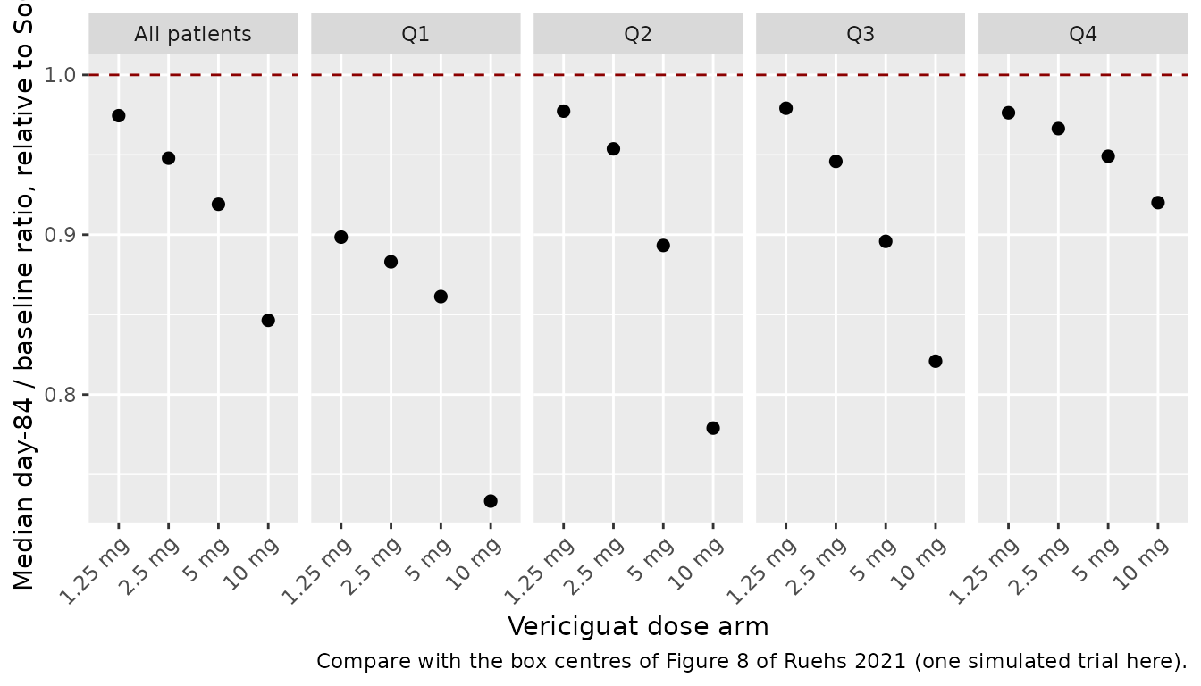
The Figure 8 box centres, read from the published figure, fall from about 0.97 (1.25 mg) to 0.83 (10 mg) for all patients, and the 10 mg effect weakens from about 0.77 in Q1 to 0.89 in Q4.
fig8_ref <- tibble::tribble(
  ~quartile, ~arm, ~digitised,
  "All patients", "1.25 mg", 0.97,
  "All patients", "2.5 mg", 0.95,
  "All patients", "5 mg", 0.90,
  "All patients", "10 mg", 0.83,
  "Q1", "10 mg", 0.77,
  "Q4", "10 mg", 0.89
)
fig8_cmp <- fig8_ref |>
  inner_join(fig8_med |> mutate(arm = as.character(arm), quartile = as.character(quartile)),
    by = c("quartile", "arm")
  ) |>
  mutate(delta = rel_soc - digitised)

fig8_cmp |>
  select(quartile, arm, digitised, rel_soc, n) |>
  rename(
    "Stratum" = quartile, "Arm" = arm,
    "Figure 8 (digitised)" = digitised, "Simulated" = rel_soc, "Patients" = n
  ) |>
knitr::kable(digits = 3, caption = "Figure 8 ratio to standard of care at day 84.")| Stratum | Arm | Figure 8 (digitised) | Simulated | Patients |
|---|---|---|---|---|
| All patients | 1.25 mg | 0.97 | 0.975 | 400 |
| All patients | 2.5 mg | 0.95 | 0.948 | 400 |
| All patients | 5 mg | 0.90 | 0.919 | 400 |
| All patients | 10 mg | 0.83 | 0.846 | 400 |
| Q1 | 10 mg | 0.77 | 0.733 | 93 |
| Q4 | 10 mg | 0.89 | 0.920 | 102 |
NT-proBNP by baseline quartile (Figure 6)
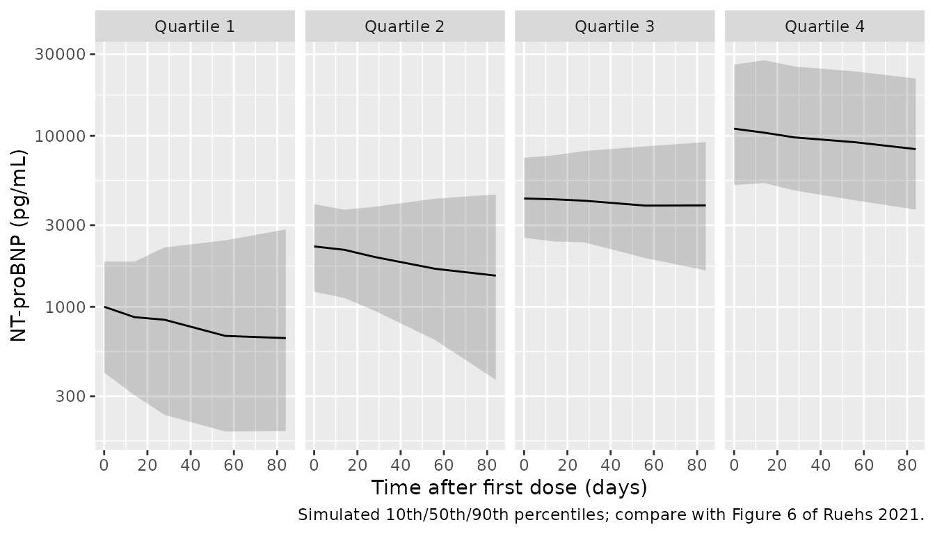
Figure 6 is a VPC of observed NT-proBNP by baseline quartile, pooling the five arms. The simulated 10th, 50th and 90th percentiles below use the same virtual patients with the log-scale residual error of Table 3 added.
set.seed(20210406)
sim_pd |>
  inner_join(bl_tbl |> rename(bl0 = bl), by = "id") |>
  filter(ntprobnp > 0) |>
  mutate(
    quartile = cut(bl0, c(0, 1559, 3000, 6246, Inf), labels = paste("Quartile", 1:4)),
    obs = ntprobnp * exp(rnorm(n(), 0, 0.38079))
  ) |>
  group_by(quartile, day = time / 24) |>
  summarise(
    q10 = quantile(obs, 0.1), q50 = median(obs), q90 = quantile(obs, 0.9),
    .groups = "drop"
  ) |>
  ggplot(aes(day, q50)) +
  geom_ribbon(aes(ymin = q10, ymax = q90), alpha = 0.2) +
  geom_line() +
  facet_wrap(~quartile, nrow = 1) +
  scale_y_log10() +
  labs(
    x = "Time after first dose (days)", y = "NT-proBNP (pg/mL)",
    caption = "Simulated 10th/50th/90th percentiles; compare with Figure 6 of Ruehs 2021."
  )
Assumptions and deviations
- Which PK drives the PK/PD model. The NT-proBNP model is packaged with the PK base model (Table 1), as the paper states and as the Figure 7b replication confirms: the final covariate model’s typical PK gives values about 15% lower. In the original analysis the PK/PD exposure came from each patient’s individual PK estimates; the packaged model instead carries the base model’s between-subject variability so it can simulate new patients.
-
24-h AUC. The paper drove kin with “the 24-h AUC
updated at 24-h intervals from the first vericiguat dose”, a step
function precomputed from the individual PK. rxode2 has no delay
operator to form a rolling 24-h integral, so the packaged model uses the
continuous
24 * C(t)(mg*h/L), whose average over any dosing interval equals that interval’s AUC. With an NT-proBNP turnover half-life of weeks, the difference is within the 1-3% agreement with Figure 7b shown above. - Titration. Figure 7 is reproduced with the study titration (2.5 mg for 2 weeks, 5 mg for 2 weeks, then 10 mg); dosing 10 mg from day 0 does not reproduce it (table above).
- Negative production rate at low baselines. As printed, Eq. 6 gives kin <= 0 for an individual baseline below exp(8.03 - 1/0.347) = 172 pg/mL; NT-proBNP then declines towards and below zero. The observed baselines reached 94.1 pg/mL and the paper does not say how this was handled. The equation is packaged as printed; with the published baseline variability about 0.15% of simulated patients fall in this range. Users simulating low-baseline patients should be aware of it.
- Bilirubin exponent. Table 2 gives -0.072 for theta CL,bilirubin and the footnote equation -0.075; the fitted-estimate table is used. The footnote equation also prints V/F as 3.43 L, a typo for the Table 2 value 34.3 L.
- Dose-bioavailability prose. Section 3.3 describes F falling “from 100% at 1.25 mg to 89% at 2.5 mg, 79% at 5 mg, and 71% at 10 mg”, which is not the ratio of the Table 2 estimates (1/1.08 = 93%, 80%, 73%). The Table 2 values are used; they reproduce the ratio of the ESM Table 4 dose-normalised geometric-mean AUCs (73% at 10 mg vs 1.25 mg), whereas the prose “82%” for that ratio does not.
- Dose step function. The paper estimates F at the studied dose levels only. The packaged model applies the 1.25 mg value at or below 1.25 mg and the 10 mg value above 5 mg (including doses above 10 mg, which were not studied).
- ATRT confidence interval. Table 3 prints the bootstrap 95% CI of ATRT as 0.024-0.360, which excludes the estimate 0.0176; it is presumably 0.0024-0.0360. The point estimate is confirmed by the Figure 7b replication.
- Covariate units. The paper does not print units for bilirubin and albumin; the reference values 0.6 and 4.0 are read as mg/dL and g/dL, and the packaged model takes the library’s SI units (umol/L, g/L) and converts. “Standardized creatinine clearance” is the Cockcroft-Gault clearance standardized to 70 kg body weight (the paper’s reference 28), not a BSA-normalised value.
- IIV of the final PK model. The final-model variances are the omega^2 values printed for the final run in ESM Table 3 (ka 0.867, CL/F 0.061, V/F 0.043); they reproduce the Table 2 CVs.
-
Residual error. The PK models use the combined
proportional plus additive error with separately estimated sigmas
(Tables 1-2 footnotes give each as SQRT(SIGMA^2)). NT-proBNP was
modelled after log transformation with an additive error, packaged as
lnorm(). - Virtual cohort covariates. The paper prints no demographics. The PK cohort centres each covariate on its Table 2 footnote median with assumed spreads: body weight log-normal (SD 0.2 on the log scale, 40-150 kg), age normal (SD 11 years, 23-95), 25% female, bilirubin log-normal (SD 0.5), standardized creatinine clearance log-normal (SD 0.3, 20-250 mL/min), and albumin normal (SD 0.4 g/dL, 2.5-5.5). Out-of-range draws are redrawn, not clamped.
- Figure 8. Reference values are box centres read from the published figure (about +/-0.01). One simulated trial of 400 patients shared across arms is compared with the paper’s 500 repeated trials, and residual error is not included in the ratio.
- Blood pressure and heart rate. The paper’s hemodynamic analyses are linear regressions of the change in systolic blood pressure on Cmax (ESM Table 5), not a dynamic model, and are not packaged.