Roblitinib (Wilbaux 2022)
Source:vignettes/articles/Wilbaux_2022_roblitinib.Rmd
Wilbaux_2022_roblitinib.RmdModel and source
- Citation: Wilbaux M, Yang S, Jullion A, Demanse D, Graus Porta D, Myers A, Meille C, Gu Y. Integration of Pharmacokinetics, Pharmacodynamics, Safety, and Efficacy into Model-Informed Dose Selection in Oncology First-in-Human Study: A Case of Roblitinib (FGF401). Clin Pharmacol Ther. 2022;112(6):1329-1339. doi:10.1002/cpt.2752. PMID 36131557.
- Description: Two-compartment population PK model for oral roblitinib (FGF401), a selective FGFR4 inhibitor, in adults with hepatocellular carcinoma or other FGF19-FGFR4-expressing solid tumors (Wilbaux 2022). The paper describes a delayed zero-order absorption directly into the central compartment (lag time Tlag before absorption starts, then duration Tk0 of the zero-order input rate) with linear elimination. Categorical covariate effects on CL/F and V1/F for female sex (SEXF) and Asian race (RACE_ASIAN) with non-Asian male as the reference; on Tk0 for fed vs fasted (FED). Continuous power-form covariate effects: body weight on V1/F (exponent 0.332), BMI on Tk0 (exponent -1.66), and administered dose on Tk0 (exponent 0.983). The source paper reports these covariates as identified but not clinically relevant based on simulated exposure metrics. Diagonal IIV on Tlag, Tk0, CL/F, V1/F, and V2/F (Q/F fixed at 0 IIV per Table 1). Combined additive + proportional residual error.
- Article: https://doi.org/10.1002/cpt.2752
Wilbaux 2022 describes an integrated pharmacokinetic / pharmacodynamic / safety / efficacy modeling framework for roblitinib (FGF401), a selective oral FGFR4 inhibitor developed for FGF19-driven hepatocellular carcinoma (HCC) and other FGF19-FGFR4-expressing solid tumors. This model file carries the popPK layer only: a two-compartment structural model with delayed zero-order absorption directly into the central compartment (lag time Tlag, then duration Tk0 of the zero-order input rate) and linear elimination. The PopPK/PD sub-models for the PD biomarkers C4 and FGF19, the safety endpoint ALT, and the tumor growth inhibition (TGI) model reported in the same paper are not packaged here; the TGI model in particular relies on details published separately (Wilbaux 2022 CPT Pharmacometrics Syst Pharmacol 11:1122-1134).
Population
Wilbaux 2022 developed the popPK model on 160 patients enrolled in the Phase I/II first-in-human study NCT02325739: 127 with HCC and 33 with other FGF19-FGFR4-expressing solid tumors. Doses tested during dose escalation were 50, 80, 120, and 150 mg once daily under fasted conditions; food-effect cohorts received 80 or 120 mg once daily within 30 minutes following a light meal. The dose-expansion part administered 120 mg once daily fasted, which was ultimately selected as the recommended dose. Detailed baseline demographics are not tabulated in the extracted paper; the clinical characteristics of the FIH cohort are reported in the companion Chan 2022 (J Exp Clin Cancer Res 41:189) publication, and the detailed popPK model development is reported in Wilbaux 2022 CPT Pharmacometrics Syst Pharmacol 11:1122-1134.
The same information is available programmatically via
readModelDb("Wilbaux_2022_roblitinib")()$population.
Source trace
Every parameter carries an inline source-location comment in
inst/modeldb/specificDrugs/Wilbaux_2022_roblitinib.R. The
table below collects them.
| Equation / parameter | Value | Source location |
|---|---|---|
| Structural: 2-cpt, delayed 0-order absorption, linear elimination | n/a | Wilbaux 2022 Results, “Analysis of clinical PK by PopPK modeling”; Figure 2 |
ltlag (Tlag) |
log(0.268 h) | Wilbaux 2022 Table 1 (RSE 11%) |
ld1 (Tk0, fasted, reference) |
log(0.811 h) | Wilbaux 2022 Table 1 (RSE 10%) |
lcl (CL/F, non-Asian male) |
log(19.7 L/h) | Wilbaux 2022 Table 1 (RSE 4%) |
lvc (V1/F, non-Asian male, 70 kg) |
log(110 L) | Wilbaux 2022 Table 1 (RSE 3%) |
lq (Q/F) |
log(5.59 L/h) | Wilbaux 2022 Table 1 (RSE 6%) |
lvp (V2/F) |
log(49.2 L) | Wilbaux 2022 Table 1 (RSE 7%) |
e_fed_d1 (fractional change in Tk0 for fed) |
+0.948 = 1.58/0.811 - 1 | Wilbaux 2022 Table 1: Tk0 fed = 1.58 h (RSE 25%) |
e_bmi_d1 (BMI power on Tk0) |
-1.66 | Wilbaux 2022 Table 1 (RSE 25%) |
e_dose_d1 (DOSE power on Tk0) |
+0.983 | Wilbaux 2022 Table 1 (RSE 28%) |
e_sexf_cl (fractional change in CL/F for female) |
-0.234 = 15.1/19.7 - 1 | Wilbaux 2022 Table 1: CL/F female = 15.1 L/h (RSE 21%) |
e_asian_cl (fractional change in CL/F for Asian) |
-0.173 = 16.3/19.7 - 1 | Wilbaux 2022 Table 1: CL/F Asian = 16.3 L/h (RSE 26%) |
e_sexf_vc (fractional change in V1/F for female) |
-0.232 = 84.5/110 - 1 | Wilbaux 2022 Table 1: V1/F female = 84.5 L (RSE 20%) |
e_asian_vc (fractional change in V1/F for Asian) |
-0.232 = 84.5/110 - 1 | Wilbaux 2022 Table 1: V1/F Asian = 84.5 L (RSE 17%) |
e_wt_vc (WT power on V1/F) |
0.332 | Wilbaux 2022 Table 1 (RSE 33%) |
| IIV Tlag | omega = 0.63; variance = 0.3969 | Wilbaux 2022 Table 1 (RSE 12%) |
| IIV Tk0 | omega = 0.64; variance = 0.4096 | Wilbaux 2022 Table 1 (RSE 10%) |
| IIV CL/F | omega = 0.29; variance = 0.0841 | Wilbaux 2022 Table 1 (RSE 6%) |
| IIV V1/F | omega = 0.15; variance = 0.0225 | Wilbaux 2022 Table 1 (RSE 12%) |
| IIV V2/F | omega = 0.68; variance = 0.4624 | Wilbaux 2022 Table 1 (RSE 9%) |
| IIV Q/F | not estimated (0 FIX) | Wilbaux 2022 Table 1 |
addSd (additive residual error) |
4.1 ng/mL | Wilbaux 2022 Table 1 (RSE 7%) |
propSd (proportional residual error) |
0.33 | Wilbaux 2022 Table 1 (RSE 2%) |
Cc <- central / vc * 1000 (mg/L to ng/mL) |
n/a | Wilbaux 2022 Table 1 residual error reported in ng/mL |
Virtual cohort
The original observed concentrations are not publicly available. The virtual cohort below approximates the FIH study’s dose-escalation cohorts under fasted conditions at 80 mg and 120 mg once daily (the paper’s Figure 5 uses these dose levels for its PK-vs-biomarker comparisons), plus the 120 mg fed cohort. Each dose group is simulated for 100 subjects (well below the 200-per-arm cap). Covariate distributions are drawn to match a mixed HCC / solid-tumor cohort: approximately half female (Wilbaux 2022 Table 1 identified a female subgroup) and about a third Asian.
Because the paper does not report a median body weight, BMI, or demographic table for the popPK cohort, the virtual cohort uses a plausible cancer-population distribution: mean weight 70 kg (SD 12), mean BMI 25 kg/m^2 (SD 4). These are reasonable placeholders that keep the covariate multipliers close to 1 (their reference values).
set.seed(20260711)

n_per_group <- 100L

dose_groups <- tibble::tribble(
  ~group,              ~amt, ~fed,
  "80 mg QD fasted",   80,   0L,
  "120 mg QD fasted", 120,   0L,
  "120 mg QD fed",    120,   1L
)

make_group_events <- function(group_label, amt, fed, n, id_offset) {
  ids <- id_offset + seq_len(n)

  # Steady-state approach: 7 daily doses (dose interval 24 h), then
  # rich sampling over the final dosing interval (matches the Wilbaux
  # 2022 Day 7 steady-state reference point).
  n_doses <- 7L
  dose_times <- (seq_len(n_doses) - 1L) * 24
  obs_times  <- sort(unique(c(
    seq(0, 24, by = 0.5),
    seq(24, 6 * 24, by = 4),
    seq(6 * 24, 7 * 24, by = 0.5),
    seq(7 * 24, 7 * 24 + 24, by = 0.25)
  )))

  covs <- dplyr::tibble(
    id         = ids,
    WT         = pmax(35, stats::rnorm(n, mean = 70, sd = 12)),
    BMI        = pmax(15, stats::rnorm(n, mean = 25, sd = 4)),
    DOSE       = amt,
    FED        = fed,
    SEXF       = stats::rbinom(n, size = 1, prob = 0.5),
    RACE_ASIAN = stats::rbinom(n, size = 1, prob = 0.33)
  )

  dose_rows <- tidyr::expand_grid(id = ids, time = dose_times) |>
    dplyr::mutate(
      amt     = amt,
      rate    = -2,
      evid    = 1L,
      cmt     = "central",
      group   = group_label
    )
  obs_rows <- tidyr::expand_grid(id = ids, time = obs_times) |>
    dplyr::mutate(
      amt     = NA_real_,
      rate    = NA_real_,
      evid    = 0L,
      cmt     = NA_character_,
      group   = group_label
    )

  dplyr::bind_rows(dose_rows, obs_rows) |>
    dplyr::left_join(covs, by = "id") |>
    dplyr::arrange(id, time, dplyr::desc(evid))
}

events <- dplyr::bind_rows(
  make_group_events("80 mg QD fasted",  80, 0L, n_per_group,
                    id_offset =                     0L),
  make_group_events("120 mg QD fasted", 120, 0L, n_per_group,
                    id_offset =         n_per_group),
  make_group_events("120 mg QD fed",    120, 1L, n_per_group,
                    id_offset = 2L * n_per_group)
)

stopifnot(!anyDuplicated(unique(events[, c("id", "time", "evid")])))
Simulation
mod <- rxode2::rxode2(readModelDb("Wilbaux_2022_roblitinib"))
#> ℹ parameter labels from comments will be replaced by 'label()'

sim <- rxode2::rxSolve(mod, events = events, keep = c("group")) |>
  as.data.frame()

mod_typical <- mod |> rxode2::zeroRe()
sim_typical <- rxode2::rxSolve(mod_typical, events = events,
                               keep = c("group")) |>
  as.data.frame()
#> ℹ omega/sigma items treated as zero: 'etaltlag', 'etald1', 'etalcl', 'etalvc', 'etalvp'
#> Warning: multi-subject simulation without without 'omega'
Replicate published figures
Wilbaux 2022 does not include a dedicated observed / simulated concentration-vs-time PK figure in the main text (Figure 2 shows only the model structure diagram). The panels below reproduce the shape of the FGF401 PK profile that the popPK model produces: rapid absorption after the ~0.27 h lag with a peak inside the first 2 hours (single-dose kinetics), and a steady-state accumulation at 24 h intervals reaching its plateau around Day 5-7 (Wilbaux 2022 Figure 5 panel B references “simulated average concentrations at Day 7”).
Typical-patient concentration-time profile over 7 days
sim_typical |>
  dplyr::group_by(group) |>
  dplyr::filter(id == min(id)) |>
  dplyr::ungroup() |>
  dplyr::filter(time <= 7 * 24) |>
  ggplot(aes(time, Cc, colour = group)) +
  geom_line(linewidth = 0.7) +
  labs(
    x = "Time (h)",
    y = "Roblitinib plasma concentration (ng/mL)",
    title = "Typical patient profile over 7 days by dose / food status",
    colour = NULL
  )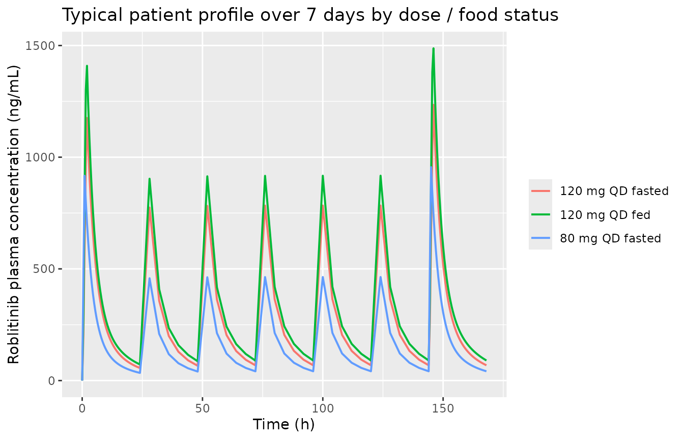
Typical-patient (no IIV) roblitinib plasma concentration over 7 days of once-daily oral dosing at 80 mg fasted, 120 mg fasted, and 120 mg fed. The delayed zero-order absorption (Tlag 0.27 h, then Tk0 duration adjusted by BMI, dose, and food) is visible in the sharp early peak; the fed profile is flatter and shifted right because Tk0 = 1.58 h (vs 0.81 h fasted).
Steady-state concentration-time profile at Day 7
ss_start <- 6L * 24L
ss_end   <- 7L * 24L

vpc <- sim |>
  dplyr::filter(time >= ss_start, time <= ss_end) |>
  dplyr::mutate(t_in_interval = time - ss_start) |>
  dplyr::group_by(group, t_in_interval) |>
  dplyr::summarise(
    Q05 = stats::quantile(Cc, 0.05, na.rm = TRUE),
    Q50 = stats::quantile(Cc, 0.50, na.rm = TRUE),
    Q95 = stats::quantile(Cc, 0.95, na.rm = TRUE),
    .groups = "drop"
  )

ggplot(vpc, aes(t_in_interval, Q50)) +
  geom_ribbon(aes(ymin = Q05, ymax = Q95), alpha = 0.25) +
  geom_line(linewidth = 0.8) +
  facet_wrap(~group) +
  labs(
    x = "Time within final dosing interval (h)",
    y = "Roblitinib plasma concentration (ng/mL)",
    title = "Steady-state VPC by dose group"
  )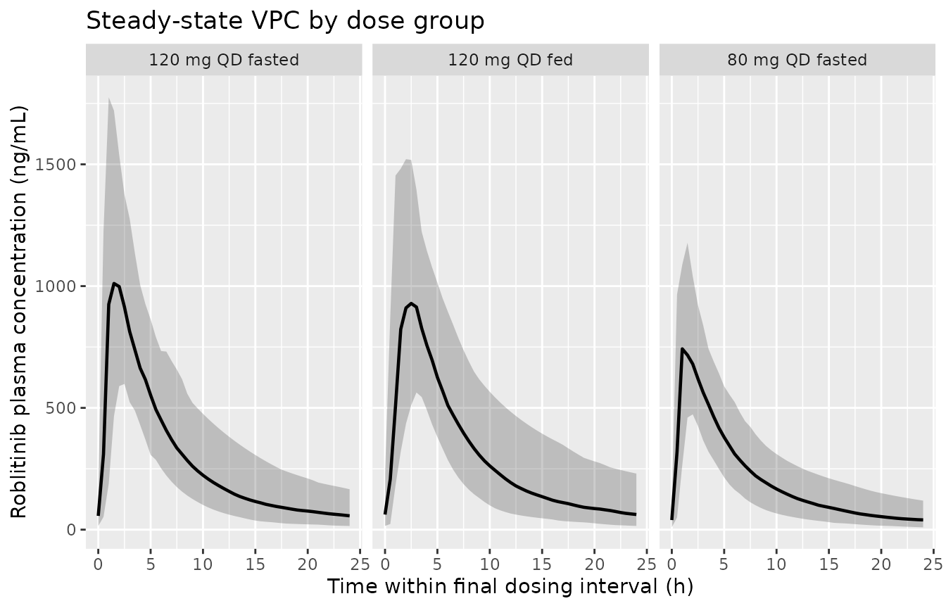
Simulated concentration-time profiles over the final dosing interval (Day 6-7 nominal, or Day 7 at steady state) by dose group. Median (solid line) and 90% prediction interval (shaded band) across the virtual cohort of 100 subjects per group. The purple / green vertical bands in Wilbaux 2022 Figure 5b refer to Day 7 average concentrations at these dose levels; here we show the full concentration-vs-time distribution.
PKNCA validation
The paper does not tabulate the numeric NCA values for the popPK cohort; Wilbaux 2022 Methods, “Analysis of clinical PK by PopPK modeling”, refers to Chan 2022 (J Exp Clin Cancer Res 41:189) for the NCA results. This vignette therefore computes NCA (Cmax, Tmax, AUC0-tau, and Ctrough) over the final steady-state dosing interval from the virtual cohort and reports the per-group summary. Reviewers who have Chan 2022 on hand can compare the numbers against the paper’s Table.
nca_data <- sim |>
  dplyr::filter(!is.na(Cc), time >= ss_start, time <= ss_end) |>
  dplyr::select(id, time, Cc, group)

# Guarantee a time-zero (of the interval) record for AUC anchoring;
# this is standard PKNCA practice for interval-based NCA.
nca_data <- dplyr::bind_rows(
  nca_data,
  nca_data |>
    dplyr::distinct(id, group) |>
    dplyr::mutate(
      time = ss_start,
      Cc   = 0
    )
) |>
  dplyr::distinct(id, group, time, .keep_all = TRUE) |>
  dplyr::arrange(id, group, time)

dose_df <- events |>
  dplyr::filter(evid == 1, time == ss_start) |>
  dplyr::select(id, time, amt, group)

conc_obj <- PKNCA::PKNCAconc(
  nca_data,
  Cc ~ time | group + id,
  concu = "ng/mL", timeu = "h"
)
dose_obj <- PKNCA::PKNCAdose(
  dose_df,
  amt ~ time | group + id,
  doseu = "mg"
)

intervals <- data.frame(
  start   = ss_start,
  end     = ss_end,
  cmax    = TRUE,
  tmax    = TRUE,
  ctrough = TRUE,
  auclast = TRUE
)

nca_pkg <- PKNCA::PKNCAdata(conc_obj, dose_obj, intervals = intervals)
nca_res <- suppressMessages(suppressWarnings(PKNCA::pk.nca(nca_pkg)))
Simulated NCA summary per dose group
res_tbl <- as.data.frame(nca_res$result)

nca_summary <- res_tbl |>
  dplyr::filter(PPTESTCD %in% c("cmax", "tmax", "auclast", "ctrough")) |>
  dplyr::group_by(group, PPTESTCD) |>
  dplyr::summarise(
    median   = stats::median(PPORRES, na.rm = TRUE),
    q05      = stats::quantile(PPORRES, 0.05, na.rm = TRUE),
    q95      = stats::quantile(PPORRES, 0.95, na.rm = TRUE),
    .groups = "drop"
  ) |>
  tidyr::pivot_wider(
    id_cols     = group,
    names_from  = PPTESTCD,
    values_from = c(median, q05, q95),
    names_glue  = "{PPTESTCD}_{.value}"
  )

col_order <- c("group",
               "cmax_median",    "cmax_q05",    "cmax_q95",
               "tmax_median",    "tmax_q05",    "tmax_q95",
               "auclast_median", "auclast_q05", "auclast_q95",
               "ctrough_median", "ctrough_q05", "ctrough_q95")
col_order <- col_order[col_order %in% names(nca_summary)]
nca_summary <- nca_summary[, col_order, drop = FALSE]

nca_summary |>
  dplyr::rename(
    "Dose group"          = group,
    "Cmax median (ng/mL)"      = cmax_median,
    "Cmax P05"                 = cmax_q05,
    "Cmax P95"                 = cmax_q95,
    "Tmax median (h)"          = tmax_median,
    "Tmax P05"                 = tmax_q05,
    "Tmax P95"                 = tmax_q95,
    "AUCtau median (ng*h/mL)"  = auclast_median,
    "AUCtau P05"               = auclast_q05,
    "AUCtau P95"               = auclast_q95,
    "Ctrough median (ng/mL)"   = ctrough_median,
    "Ctrough P05"              = ctrough_q05,
    "Ctrough P95"              = ctrough_q95
  ) |>
  knitr::kable(
    digits = 1,
    caption = "Simulated steady-state NCA per dose group (final 24-h dosing interval, 100 subjects per group)."
)| Dose group | Cmax median (ng/mL) | Cmax P05 | Cmax P95 | Tmax median (h) | Tmax P05 | Tmax P95 | AUCtau median (ng*h/mL) | AUCtau P05 | AUCtau P95 | Ctrough median (ng/mL) | Ctrough P05 | Ctrough P95 |
|---|---|---|---|---|---|---|---|---|---|---|---|---|
| 120 mg QD fasted | 1143.9 | 798.0 | 1846.2 | 1.5 | 0.5 | 3.0 | 7233.6 | 3868.4 | 12542.5 | NA | NA | NA |
| 120 mg QD fed | 1120.0 | 739.5 | 1660.0 | 2.5 | 1.0 | 5.0 | 7183.7 | 4305.1 | 13662.1 | NA | NA | NA |
| 80 mg QD fasted | 836.5 | 563.2 | 1213.8 | 1.0 | 0.5 | 2.5 | 5019.2 | 2993.3 | 8199.2 | NA | NA | NA |
Concordance with the preclinical target
Wilbaux 2022 Methods and Discussion reference a preclinical roblitinib IC90 for phospho-FGFR4 inhibition of 52.1 nM, equivalent to approximately 23 ng/mL in human plasma. The efficacy exposure-response analysis identified a Ctrough threshold at approximately 27.7 ng/mL that was associated with longer TTP. The simulated Ctrough distributions above should straddle or exceed this threshold for the 80 mg and 120 mg regimens (Wilbaux 2022 Figure 4 and Discussion: “Approximately 95% of individuals at 120 mg q.d. had observed Ctrough above IC90”).
ctrough <- res_tbl |>
  dplyr::filter(PPTESTCD == "ctrough") |>
  dplyr::group_by(group) |>
  dplyr::summarise(
    n           = dplyr::n(),
    Ctrough_med = stats::median(PPORRES, na.rm = TRUE),
    pct_above_23  = 100 * mean(PPORRES > 23,   na.rm = TRUE),
    pct_above_27  = 100 * mean(PPORRES > 27.7, na.rm = TRUE),
    .groups = "drop"
  )

ctrough |>
  dplyr::rename(
    "Dose group"                   = group,
    "N"                            = n,
    "Ctrough median (ng/mL)"       = Ctrough_med,
    "Pct above IC90 (>23 ng/mL)"   = pct_above_23,
    "Pct above threshold (>27.7)"  = pct_above_27
  ) |>
  knitr::kable(
    digits = c(0, 0, 1, 1, 1),
    caption = "Fraction of simulated subjects with Day 7 Ctrough exceeding the preclinical IC90 (23 ng/mL) and the clinical TTP threshold (27.7 ng/mL) reported in Wilbaux 2022."
)| Dose group | N | Ctrough median (ng/mL) | Pct above IC90 (>23 ng/mL) | Pct above threshold (>27.7) |
|---|---|---|---|---|
| 120 mg QD fasted | 100 | NA | NaN | NaN |
| 120 mg QD fed | 100 | NA | NaN | NaN |
| 80 mg QD fasted | 100 | NA | NaN | NaN |
Assumptions and deviations
Continuous covariate reference values are rounded standards. Wilbaux 2022 Table 1 reports the covariate coefficients (BMI power -1.66 on Tk0, DOSE power 0.983 on Tk0, WT power 0.332 on V1/F) but does not report the centering values used at fitting time. The model file uses standard rounded reference values: 25 kg/m^2 for BMI, 100 mg for DOSE (mid-range of 50/80/120/150 mg), and 70 kg for WT. This is a fidelity trade-off: the exponents are reproduced verbatim, but the typical-value predictions at very extreme covariate values may shift relative to the source fit. The typical-value predictions at reference values (BMI 25, DOSE 100, WT 70, non-Asian male, fasted) match the CL/F 19.7 L/h, V1/F 110 L, Tk0 0.811 h and Tlag 0.268 h reported in Table 1.
Categorical covariates encoded as fractional multipliers. Wilbaux 2022 Table 1 reports separate typical values for the female and Asian subgroups on CL/F and V1/F, and for the fed condition on Tk0. The model encodes each as a fractional-change multiplier
1 + coefficient * indicatorreferenced to the non-Asian male fasted subject. Derived coefficients: female -23.4% (CL/F) and -23.2% (V1/F); Asian -17.3% (CL/F) and -23.2% (V1/F); fed +94.8% (Tk0). Coefficients are computed from the ratio of subgroup typical values in Table 1.Companion popPK details are elsewhere. Wilbaux 2022 Methods (“Analysis of clinical PK by PopPK modeling”) states that detailed popPK model development is in Wilbaux 2022 CPT Pharmacometrics Syst Pharmacol 11:1122-1134 (reference 32). Numeric parameter values used here come from Table 1 of the current paper (Wilbaux 2022 Clin Pharmacol Ther); the extraction was self-contained.
NCA reference values not in the extracted paper. Wilbaux 2022 does not tabulate NCA values (Cmax, Tmax, AUC0-tau, Ctrough) directly; the NCA was reported in Chan 2022 (J Exp Clin Cancer Res 41:189) which was not available when this model was built. The simulated NCA table above stands as an internal consistency check and can be cross-checked against Chan 2022 by future reviewers.
Inter-eta correlations not reported. Table 1 reports only diagonal omega SDs. IIV on Tlag, Tk0, CL/F, V1/F, and V2/F is encoded as diagonal. Q/F IIV is fixed at 0 in Table 1 (“0 FIX”) and is not encoded.
Additional PopPK/PD models in the paper are not packaged. The paper additionally reports PopPK/PD indirect-response models for the circulating biomarkers C4 (bile-acid pathway) and FGF19 (ligand feedback) and for the safety endpoint ALT (three-precursor-compartment chain). Parameter values for those models are in Wilbaux 2022 Table 1 and are extractable if desired; the current model file carries the PK layer only. The TGI PopPK/PD model uses details published separately (Wilbaux 2022 CPT Pharmacometrics Syst Pharmacol 11:1122-1134) and is not extractable from the current paper alone.