Paracetamol food effects in beagle dogs and human adults (Gasthuys 2023)
Source:vignettes/articles/Gasthuys_2023_paracetamol.Rmd
Gasthuys_2023_paracetamol.RmdModel and source
Gasthuys 2023 asked whether population PK built from beagle dogs and from human adults can predict the effect of food on paracetamol exposure in children. Two independent models were fitted, one per species, and the paper contributes both to nlmixr2lib:
modellib("Gasthuys_2023_paracetamol_dog")– two-compartment, sequential zero-order then first-order absorption, absolute bioavailability F estimable because an intravenous occasion was run.modellib("Gasthuys_2023_paracetamol_human")– one-compartment, dual zero-order input function with a lag on the second input, apparent (CL/F, Vd/F) disposition because no intravenous arm was run.Citation: Gasthuys E, Sandra L, Statelova M, Vertzoni M, Vermeulen A. The Use of Population Pharmacokinetics to Extrapolate Food Effects from Human Adults and Beagle Dogs to the Pediatric Population Illustrated with Paracetamol as a Test Case. Pharmaceuticals. 2024;17(1):53. doi:10.3390/ph17010053 (published online 2023-12-28). Beagle dog study design and data originally reported in Statelova et al. 2023 (cited as ref [14]).
Article: https://doi.org/10.3390/ph17010053
Supplement (individual fits, goodness-of-fit and IWRES plots only; no parameter values): https://www.mdpi.com/article/10.3390/ph17010053/s1
This vignette carries two findings that a reader should see before using either model. Both are worked quantitatively below and summarised under Assumptions and deviations:
- The 70 kg allometric reference of the paper’s Eq. 1 cannot be the reference used for the beagle-dog fit – taking it literally overpredicts the dogs’ own observed AUC roughly six-fold. The dog model therefore normalises to the 9.70 kg median dog weight.
- The published human-adult CL/F and Vd/F are mutually consistent (they give a correct 2.2 h half-life and reproduce the paper’s own Cmax:AUC ratio to about 1%) but are jointly about 2.6-fold too low to reproduce the paper’s own non-compartmental AUC at the stated 1000 mg dose. The values are encoded exactly as published and are not tuned.
Population
Beagle dogs. Six clinically healthy adult beagle dogs (median age 1.9 years, range 1.7-4.0; median body weight 9.70 kg, range 7.90-13.3 kg) contributed 575 plasma paracetamol concentrations over eight occasions in a sequential (not crossover) design spanning 50 days (Gasthuys 2023 Methods 4.1.1 and Figure 5). Each oral occasion delivered 168 mg of paracetamol (7 mL of Panadol suspension) by gavage followed by 10 mL of tap water; a single 168 mg intravenous injection was given on day 14, which is what makes the absolute bioavailability F identifiable. Prandial conditions were fasted, fasted after 0.1 M HCl/KCl pretreatment, reference meal at 100 and 200 kcal, and infant formula at 100 and 200 kcal. Assay was validated HPLC-UV with a 7.5 ng/mL limit of quantification; 1.19% of dog records were below it and were excluded before fitting.
Human adults. Eight healthy adult Caucasian men (ten enrolled, eight completed; median age 25 years, range 21-48; median body weight 81.5 kg, range 60-104; median height 1.85 m; median BMI 23.8 kg/m2) contributed 360 plasma concentrations over three occasions of a single-dose, open-label, randomised, three-period crossover study (Gasthuys 2023 Table 4 and Figure 6). Each occasion delivered a single oral 1000 mg dose (42 mL of Panadol suspension at 24 mg/mL) under one of three conditions: fasted, after a 990 kcal reference meal given 30 min before dosing, or with 800 mL of infant formula (520 kcal) split around the dose. Fifteen PK samples were taken over 0-10 h; 0.83% of records were below the limit of quantification and were excluded.
A double absorption peak or shoulder was visible in four of eight subjects on the reference-meal occasion, two of eight fasted and one of eight on infant formula; the dual input function exists to describe it. No such feature appeared in the dog profiles.
The same information is available programmatically from each model’s
population metadata, e.g.
rxode2::rxode(readModelDb("Gasthuys_2023_paracetamol_human"))$population.
Source trace
Every value below is transcribed from Gasthuys 2023 Table 3 (final
model parameter estimates, two columns: beagle dogs and human adults).
The per-value provenance is also recorded as an in-file comment on each
ini() line of
inst/modeldb/specificDrugs/Gasthuys_2023_paracetamol_dog.R
and ..._human.R. Nothing in either model is digitised from
a figure, taken from an author communication, or carried from an
upstream publication.
Beagle dog model
| Equation / parameter | Value | Source location |
|---|---|---|
logitfdepot (F) |
0.80 | Table 3, “F”, RSE 2.56% |
lka |
2.86 1/h | Table 3, “ka” , RSE 14.2% |
lvc (Vd) |
9.53 L | Table 3, “Vd”, RSE 1.55% |
lcl (CL) |
9.29 L/h | Table 3, “CL”, RSE 1.92% |
lvp (Vp) |
34.9 L | Table 3, “Vp”, RSE 4.56% |
lq (Q) |
2.82 L/h | Table 3, “Q”, RSE 0.835% |
ld1 (dT1) |
0.64 h | Table 3, “dT1”, RSE 16.1% |
e_wt_cl |
0.75 (fixed) | Table 3, “beta WTonCL = 0.75 [FIX]” |
e_wt_vc |
1 (fixed) | Table 3, “beta WTonVd = 1 [FIX]” |
e_wt_vp |
1 (fixed) | Table 3, “beta WTonVp = 1 [FIX]” |
e_wt_q |
1 (fixed) | Table 3, “beta WTonQ = 1 [FIX]” (see Errata: Methods 4.2 says 0.75) |
etalogitfdepot |
0.11 (SD) | Table 3, “IOV F”, RSE 14.3%; folded as BSV-equivalent |
etalka |
0.63 (SD) | Table 3, “IOV ka”, RSE 18.0%; folded as BSV-equivalent |
etald1 |
0.86 (SD) | Table 3, “IOV dT1”, RSE 15.2%; folded as BSV-equivalent |
addSd |
0.055 ug/mL | Table 3, “a”, RSE 9.30% |
propSd |
0.13 | Table 3, “b”, RSE 7.13% |
| Reference weight 9.70 kg | n/a | Methods 4.1.1 (“median body weight of 9.70 kg”); see Errata |
Absorption structure: zero-order into depot over dT1,
then first-order ka into central; 2-compartment
disposition |
n/a | Results 2.1, paragraph 3; Figure 2a schematic |
Allometric form theta * (WT / WTref)^beta
|
n/a | Eq. 1, Methods 4.2 |
Human adult model
| Equation / parameter | Value | Source location |
|---|---|---|
logitfrel (Bio) |
0.45 | Table 3, “Bio”, RSE 27.5% |
lka |
1.79 1/h | Table 3, “ka”, RSE 38.1% |
lvc (Vd/F) |
27.6 L | Table 3, “Vd”, RSE 2.42%, footnote * = Vd/F |
lcl (CL/F) |
8.79 L/h | Table 3, “CL”, RSE 1.99%, footnote * = CL/F |
ld1 (dT1) |
0.22 h | Table 3, “dT1”, RSE 39.2% |
ld2 (dT2) |
2.73 h | Table 3, “dT2”, RSE 34.2% |
ltlag (T2) |
0.97 h | Table 3, “T2”, RSE 31.8%; Results 2.1 “a lag time was implemented” |
e_wt_cl |
0.75 (fixed) | Table 3, “beta WTonCL = 0.75 [FIX]” |
e_wt_vc |
1 (fixed) | Table 3, “beta WTonVd = 1 [FIX]” |
etalvc |
0.098 (SD) | Table 3, “BSV Vd”, RSE 39.9% |
etalcl |
0.13 (SD) | Table 3, “BSV CL”, RSE 26.0% |
etalogitfrel |
0.69 (SD) | Table 3, “IOV Bio”, RSE 20.7%; folded as BSV-equivalent |
etalka |
0.53 (SD) | Table 3, “IOV ka”, RSE 56.4%; folded as BSV-equivalent |
etald1 |
1.58 (SD) | Table 3, “IOV dT1”, RSE 25.9%; folded as BSV-equivalent |
etald2 |
0.87 (SD) | Table 3, “IOV dT2”, RSE 22.0%; folded as BSV-equivalent |
etaltlag |
0.59 (SD) | Table 3, “IOV T2”, RSE 38.3%; folded as BSV-equivalent |
addSd |
0.094 ug/mL | Table 3, “a”, RSE 23.9% |
propSd |
0.094 | Table 3, “b”, RSE 11.2% |
| Reference weight 70 kg | n/a | Eq. 1 (“typical population value … in a 70 kg individual”) |
Absorption structure: Bio zero-order into depot over
dT1, (1 - Bio) zero-order into depot2 over dT2 after lag
T2, common ka into central; 1-compartment disposition |
n/a | Results 2.1, paragraph 4; Figure 2b schematic |
Reference values used for validation are Gasthuys 2023 Table 1 (six dog conditions) and Table 2 (three human conditions), both reported as mean +/- SD except Tmax, which is median [range].
Virtual cohort
The original observed concentrations are not public (Gasthuys 2023 Data Availability Statement: “available on request from the corresponding author”), so the figures use virtual cohorts whose body-weight distributions span the published ranges.
Neither final model retained a food covariate – “No significant food effect could be retained during the covariate analysis in both species” (Gasthuys 2023 Discussion). A single oral arm per species therefore constitutes the model’s prediction for every prandial condition the paper studied, and that is exactly how the comparison tables below are laid out.
# set.seed() seeds R's RNG only. rxode2's simulation RNG is partitioned per
# solver thread, so this cohort is reproducible on a given machine and
# different on a machine with a different thread count. Every assertion below
# is written to hold for any cohort these models can produce; the tight gates
# are all on typical-value (zeroRe) quantities, which are deterministic.
set.seed(20231228)

n_per_arm <- 100L

make_arm <- function(n, wt_min, wt_max, dose, cmts, label, t_obs, id_offset = 0L) {
  subj <- tibble(
    id = id_offset + seq_len(n),
    WT = runif(n, wt_min, wt_max),
    treatment = label
  )
  doses <- subj |>
    tidyr::crossing(cmt = cmts) |>
    mutate(time = 0, amt = dose, evid = 1L)
  obs <- subj |>
    tidyr::crossing(time = t_obs) |>
    mutate(cmt = "central", amt = NA_real_, evid = 0L)
  bind_rows(doses, obs) |>
    arrange(id, time, desc(evid)) |>
    select(id, time, amt, evid, cmt, WT, treatment)
}

# Dog observation grid: fine through the absorption peak (Tmax ~ 0.5 h), then
# coarse out to 48 h (about 4 terminal half-lives, the terminal slope being
# roughly 0.061 1/h for this 2-compartment parameterisation).
t_dog <- unique(c(seq(0, 4, by = 0.05), seq(4, 12, by = 0.25), seq(12, 48, by = 1)))

# Human observation grid: the lagged second input releases over 0.97-3.70 h, so
# resolve 0-6 h finely; 36 h is about 16 half-lives.
t_hum <- unique(c(seq(0, 6, by = 0.05), seq(6, 12, by = 0.25), seq(12, 36, by = 1)))

events_dog <- bind_rows(
  make_arm(n_per_arm, 7.90, 13.3, 168, "depot",   "Oral 168 mg", t_dog, id_offset = 0L),
  make_arm(n_per_arm, 7.90, 13.3, 168, "central", "IV 168 mg",   t_dog, id_offset = 1000L)
)

# The human dual input needs TWO dose records per administration, one per
# dosing compartment, each carrying the full amount; f(depot) = Bio and
# f(depot2) = 1 - Bio then split it.
events_hum <- make_arm(
  n_per_arm, 60, 104, 1000, c("depot", "depot2"), "Oral 1000 mg", t_hum,
  id_offset = 2000L
)

stopifnot(
  !anyDuplicated(unique(events_dog[, c("id", "time", "evid", "cmt")])),
  !anyDuplicated(unique(events_hum[, c("id", "time", "evid", "cmt")])),
  length(intersect(events_dog$id, events_hum$id)) == 0L
)
Simulation
mod_dog <- readModelDb("Gasthuys_2023_paracetamol_dog")
mod_hum <- readModelDb("Gasthuys_2023_paracetamol_human")

sim_dog <- rxode2::rxSolve(mod_dog, events = events_dog,
                           keep = c("WT", "treatment")) |>
  as.data.frame()
#> ℹ parameter labels from comments will be replaced by 'label()'
sim_hum <- rxode2::rxSolve(mod_hum, events = events_hum,
                           keep = c("WT", "treatment")) |>
  as.data.frame()
#> ℹ parameter labels from comments will be replaced by 'label()'

# Concentrations must stay strictly positive or PKNCA's log-down trapezoid
# takes log() of a negative number and returns NaN.
stopifnot(all(sim_dog$Cc[sim_dog$time > 0] > 0),
          all(sim_hum$Cc[sim_hum$time > 0] > 0))
Typical-value (no between-subject variability) solves at each species’ median body weight are used for every quantitative gate below, because they are deterministic and so can be asserted tightly.
typ_dog <- rxode2::zeroRe(rxode2::rxode(mod_dog))
#> ℹ parameter labels from comments will be replaced by 'label()'
typ_hum <- rxode2::zeroRe(rxode2::rxode(mod_hum))
#> ℹ parameter labels from comments will be replaced by 'label()'

ev_typ_dog <- rxode2::et(amt = 168, cmt = "depot") |>
  rxode2::et(seq(0, 96, by = 0.02), cmt = "central")
ev_typ_hum <- rxode2::et(amt = 1000, cmt = "depot") |>
  rxode2::et(amt = 1000, cmt = "depot2") |>
  rxode2::et(seq(0, 96, by = 0.02), cmt = "central")

trapz <- function(t, y) sum(diff(t) * (head(y, -1) + tail(y, -1)) / 2)

# Median dog weight (9.70 kg) and median adult weight (81.5 kg).
sd970 <- rxode2::rxSolve(typ_dog, ev_typ_dog, params = c(WT = 9.70),
                         returnType = "data.frame")
#> ℹ omega/sigma items treated as zero: 'etalogitfdepot', 'etalka', 'etald1'
sh815 <- rxode2::rxSolve(typ_hum, ev_typ_hum, params = c(WT = 81.5),
                         returnType = "data.frame")
#> ℹ omega/sigma items treated as zero: 'etalvc', 'etalcl', 'etalogitfrel', 'etalka', 'etald1', 'etald2', 'etaltlag'
Replicate published figures
Figure 1 / Figure 3 – plasma concentration-time profiles
Gasthuys 2023 Figure 1 shows the observed profiles and Figure 3 the prediction-corrected VPCs, both stratified by dosing condition. Because neither final model carries a food covariate, the model produces one profile per species; the panels below are the 5th, 50th and 95th simulated percentiles of that single prediction.
# Replicates the shape of Figure 1a / Figure 3a of Gasthuys 2023 (beagle dogs).
sim_dog |>
  filter(time > 0) |>
  group_by(treatment, time) |>
  summarise(Q05 = quantile(Cc, 0.05), Q50 = median(Cc),
            Q95 = quantile(Cc, 0.95), .groups = "drop") |>
  ggplot(aes(time, Q50)) +
  geom_ribbon(aes(ymin = Q05, ymax = Q95), alpha = 0.25) +
  geom_line() +
  facet_wrap(~treatment) +
  coord_cartesian(xlim = c(0, 24)) +
  scale_y_log10() +
  labs(x = "Time (h)", y = "Plasma paracetamol (ug/mL)",
       caption = "Beagle dogs, 168 mg. Replicates Figure 1a / 3a of Gasthuys 2023.")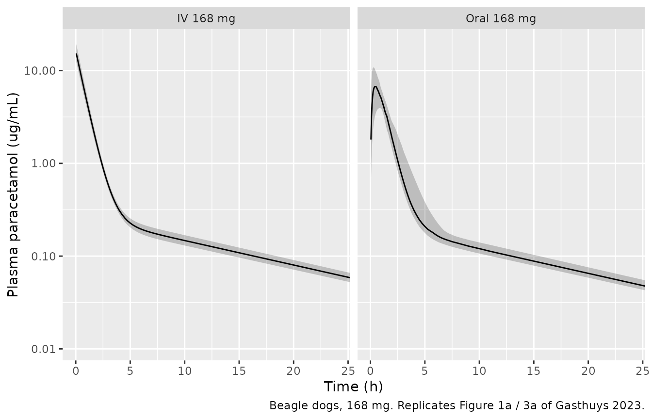
# Replicates the shape of Figure 1b / Figure 3b of Gasthuys 2023 (human adults).
sim_hum |>
  filter(time > 0) |>
  group_by(time) |>
  summarise(Q05 = quantile(Cc, 0.05), Q50 = median(Cc),
            Q95 = quantile(Cc, 0.95), .groups = "drop") |>
  ggplot(aes(time, Q50)) +
  geom_ribbon(aes(ymin = Q05, ymax = Q95), alpha = 0.25) +
  geom_line() +
  coord_cartesian(xlim = c(0, 12)) +
  labs(x = "Time (h)", y = "Plasma paracetamol (ug/mL)",
       caption = "Human adults, 1000 mg. Replicates Figure 1b / 3b of Gasthuys 2023.")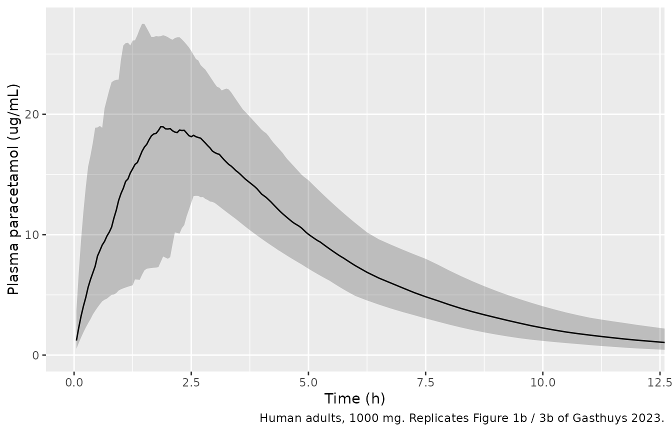
Figure 2b – the dual input function
The paper’s distinguishing structural feature is the human dual input: a fraction Bio released immediately over dT1 = 0.22 h and the remainder released over dT2 = 2.73 h starting only after a T2 = 0.97 h lag. Decomposing the typical profile into its two arms shows how the second, lagged arm produces the shoulder that Results 2.1 describes.
solve_arm <- function(frac_depot) {
  ev <- rxode2::et(amt = 1000 * frac_depot, cmt = "depot") |>
    rxode2::et(amt = 1000 * (1 - frac_depot), cmt = "depot2") |>
    rxode2::et(seq(0, 12, by = 0.02), cmt = "central")
  rxode2::rxSolve(typ_hum, ev, params = c(WT = 81.5), returnType = "data.frame")
}
# f(depot) = Bio and f(depot2) = 1 - Bio are applied by the model, so routing
# the whole dose to one compartment isolates that arm's contribution.
arm1 <- solve_arm(1)   # only the immediate (dT1) arm carries drug
#> ℹ omega/sigma items treated as zero: 'etalvc', 'etalcl', 'etalogitfrel', 'etalka', 'etald1', 'etald2', 'etaltlag'
arm2 <- solve_arm(0)   # only the lagged (dT2) arm carries drug
#> ℹ omega/sigma items treated as zero: 'etalvc', 'etalcl', 'etalogitfrel', 'etalka', 'etald1', 'etald2', 'etaltlag'

bind_rows(
  tibble(time = arm1$time, Cc = arm1$Cc, arm = "Arm 1: Bio, zero-order over dT1"),
  tibble(time = arm2$time, Cc = arm2$Cc, arm = "Arm 2: 1 - Bio, over dT2 after lag T2"),
  tibble(time = sh815$time, Cc = sh815$Cc, arm = "Total")
) |>
  filter(time <= 12) |>
  ggplot(aes(time, Cc, colour = arm, linetype = arm)) +
  geom_line(linewidth = 0.7) +
  labs(x = "Time (h)", y = "Plasma paracetamol (ug/mL)", colour = NULL,
       linetype = NULL,
       caption = "Decomposition of the Figure 2b dual input function (typical values, 81.5 kg).") +
  theme(legend.position = "bottom", legend.direction = "vertical")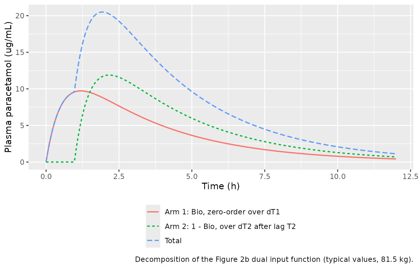
# The second arm must not start before its lag, and the first must peak first.
stopifnot(
  # Nothing from arm 2 before T2 = 0.97 h (allow one 0.02 h grid step).
  all(arm2$Cc[arm2$time < 0.95] == 0),
  # ... and something after it.
  max(arm2$Cc) > 0,
  # Arm 1 peaks earlier than arm 2 (dT1 = 0.22 h with no lag vs dT2 = 2.73 h
  # starting at 0.97 h) -- deterministic, so an exact ordering is safe here.
  arm1$time[which.max(arm1$Cc)] < arm2$time[which.max(arm2$Cc)]
)
PKNCA validation
nca_dog_conc <- sim_dog |>
  filter(!is.na(Cc)) |>
  select(id, time, Cc, treatment)
nca_dog_conc <- bind_rows(
  nca_dog_conc,
  nca_dog_conc |> distinct(id, treatment) |> mutate(time = 0, Cc = 0)
) |>
  distinct(id, treatment, time, .keep_all = TRUE) |>
  arrange(id, treatment, time)

conc_dog <- PKNCA::PKNCAconc(nca_dog_conc, Cc ~ time | treatment + id)
dose_dog <- PKNCA::PKNCAdose(
  events_dog |> filter(evid == 1, cmt %in% c("depot", "central")) |>
    select(id, time, amt, treatment),
  amt ~ time | treatment + id
)
res_dog <- PKNCA::pk.nca(PKNCA::PKNCAdata(
  conc_dog, dose_dog,
  intervals = data.frame(start = 0, end = Inf, cmax = TRUE, tmax = TRUE,
                         auclast = TRUE, aucinf.obs = TRUE, half.life = TRUE)
))
nca_hum_conc <- sim_hum |>
  filter(!is.na(Cc)) |>
  select(id, time, Cc, treatment)
nca_hum_conc <- bind_rows(
  nca_hum_conc,
  nca_hum_conc |> distinct(id, treatment) |> mutate(time = 0, Cc = 0)
) |>
  distinct(id, treatment, time, .keep_all = TRUE) |>
  arrange(id, treatment, time)

conc_hum <- PKNCA::PKNCAconc(nca_hum_conc, Cc ~ time | treatment + id)
# One dose row per subject: the two dose records are the two arms of a single
# 1000 mg administration, not two administrations.
dose_hum <- PKNCA::PKNCAdose(
  events_hum |> filter(evid == 1, cmt == "depot") |>
    select(id, time, amt, treatment),
  amt ~ time | treatment + id
)
res_hum <- PKNCA::pk.nca(PKNCA::PKNCAdata(
  conc_hum, dose_hum,
  intervals = data.frame(start = 0, end = Inf, cmax = TRUE, tmax = TRUE,
                         auclast = TRUE, aucinf.obs = TRUE, half.life = TRUE)
))
Comparison against published NCA
Because neither model retained a food covariate, the simulated column is the same prediction on every row; the spread down the reference column is the between-condition variation the models cannot reproduce by construction. That is the paper’s own conclusion (“for both the RM and the IF, the food effect at the population level is comparable”), restated as a table.
sim_dog_long <- as.data.frame(res_dog$result) |>
  filter(treatment == "Oral 168 mg",
         PPTESTCD %in% c("cmax", "tmax", "aucinf.obs")) |>
  select(id, PPTESTCD, PPORRES)

dog_published <- tibble::tribble(
  ~treatment,        ~cmax, ~tmax, ~aucinf.obs,
  "Fasted",           6.07,  0.63,  9.86,
  "Fasted HCl/KCl",   6.11,  1.00, 11.4,
  "RM100",            6.21,  0.88, 11.6,
  "RM200",            4.50,  1.50,  9.86,
  "IF100",            5.18,  1.50, 16.2,
  "IF200",            3.79,  1.75, 11.3
)

cmp_dog <- nlmixr2lib::ncaComparisonTable(
  simulated = dog_published |>
    select(treatment) |>
    tidyr::crossing(sim_dog_long),
  reference = dog_published,
  by = "treatment",
  units = c(cmax = "ug/mL", tmax = "h", aucinf.obs = "ug*h/mL"),
  tolerance_pct = 20
)
knitr::kable(
  cmp_dog, digits = 2,
  caption = paste(
    "Beagle dogs, 168 mg oral. Simulated column is one food-covariate-free",
    "prediction repeated against each published condition (Gasthuys 2023",
    "Table 1). * differs from reference by more than 20%."
  )
)| NCA parameter | treatment | Reference | Simulated | % diff |
|---|---|---|---|---|
| Cmax (ug/mL) | Fasted | 6.07 | 6.81 | +12.1% |
| Cmax (ug/mL) | Fasted HCl/KCl | 6.11 | 6.81 | +11.4% |
| Cmax (ug/mL) | RM100 | 6.21 | 6.81 | +9.6% |
| Cmax (ug/mL) | RM200 | 4.5 | 6.81 | +51.3%* |
| Cmax (ug/mL) | IF100 | 5.18 | 6.81 | +31.4%* |
| Cmax (ug/mL) | IF200 | 3.79 | 6.81 | +79.6%* |
| Tmax (h) | Fasted | 0.63 | 0.5 | -20.6%* |
| Tmax (h) | Fasted HCl/KCl | 1 | 0.5 | -50.0%* |
| Tmax (h) | RM100 | 0.88 | 0.5 | -43.2%* |
| Tmax (h) | RM200 | 1.5 | 0.5 | -66.7%* |
| Tmax (h) | IF100 | 1.5 | 0.5 | -66.7%* |
| Tmax (h) | IF200 | 1.75 | 0.5 | -71.4%* |
| AUC0-∞ (obs) (ug*h/mL) | Fasted | 9.86 | 13.5 | +36.7%* |
| AUC0-∞ (obs) (ug*h/mL) | Fasted HCl/KCl | 11.4 | 13.5 | +18.2% |
| AUC0-∞ (obs) (ug*h/mL) | RM100 | 11.6 | 13.5 | +16.2% |
| AUC0-∞ (obs) (ug*h/mL) | RM200 | 9.86 | 13.5 | +36.7%* |
| AUC0-∞ (obs) (ug*h/mL) | IF100 | 16.2 | 13.5 | -16.8% |
| AUC0-∞ (obs) (ug*h/mL) | IF200 | 11.3 | 13.5 | +19.3% |
sim_hum_long <- as.data.frame(res_hum$result) |>
  filter(PPTESTCD %in% c("cmax", "tmax", "aucinf.obs")) |>
  select(id, PPTESTCD, PPORRES)

human_published <- tibble::tribble(
  ~treatment,        ~cmax, ~tmax, ~aucinf.obs,
  "Fasted",           7.85,  1.50, 39.3,
  "Reference meal",   6.96,  2.50, 40.2,
  "Infant formula",   7.24,  4.00, 39.2
)

cmp_hum <- nlmixr2lib::ncaComparisonTable(
  simulated = human_published |>
    select(treatment) |>
    tidyr::crossing(sim_hum_long),
  reference = human_published,
  by = "treatment",
  units = c(cmax = "ug/mL", tmax = "h", aucinf.obs = "ug*h/mL"),
  tolerance_pct = 20
)
knitr::kable(
  cmp_hum, digits = 2,
  caption = paste(
    "Human adults, 1000 mg oral. Simulated column is one food-covariate-free",
    "prediction repeated against each published condition (Gasthuys 2023",
    "Table 2). * differs from reference by more than 20%."
  )
)| NCA parameter | treatment | Reference | Simulated | % diff |
|---|---|---|---|---|
| Cmax (ug/mL) | Fasted | 7.85 | 20.7 | +163.8%* |
| Cmax (ug/mL) | Reference meal | 6.96 | 20.7 | +197.5%* |
| Cmax (ug/mL) | Infant formula | 7.24 | 20.7 | +186.0%* |
| Tmax (h) | Fasted | 1.5 | 1.98 | +31.7%* |
| Tmax (h) | Reference meal | 2.5 | 1.98 | -21.0%* |
| Tmax (h) | Infant formula | 4 | 1.98 | -50.6%* |
| AUC0-∞ (obs) (ug*h/mL) | Fasted | 39.3 | 109 | +176.4%* |
| AUC0-∞ (obs) (ug*h/mL) | Reference meal | 40.2 | 109 | +170.2%* |
| AUC0-∞ (obs) (ug*h/mL) | Infant formula | 39.2 | 109 | +177.1%* |
The dog Cmax and AUC rows land within about 20-50% of the published means, which is what a single typical-value structure fitted across six prandial conditions can do. The human Cmax and AUC rows are starred at roughly +160% in every condition. That is not a transcription error; it is worked out next.
Finding 1 – the 70 kg allometric reference is falsified for the dogs
Gasthuys 2023 Eq. 1 writes the covariate model as
log(theta_i) = log(theta_70pop) + beta * log(WT_i / 70) + eta_i + eta_occ,i
and defines theta_70pop as “typical population value for
the PK parameter in a 70 kg individual”. Applied literally to the
beagle-dog column of Table 3, a 9.70 kg dog would carry
CL = 9.29 * (9.70/70)^0.75 and
Vd = 9.53 * (9.70/70).
Because the allometric factor is a pure power of
WT / WTref, the 70 kg-reference counterfactual can be
obtained from the shipped model without editing it: solving at
WT = 9.70^2 / 70 makes (WT / 9.70)^b identical
to (9.70 / 70)^b for every exponent b.
sd70 <- rxode2::rxSolve(typ_dog, ev_typ_dog, params = c(WT = 9.70^2 / 70),
                        returnType = "data.frame")
#> ℹ omega/sigma items treated as zero: 'etalogitfdepot', 'etalka', 'etald1'

dog_ref_tbl <- tibble(
  Reference = c("9.70 kg (dog median; used here)", "70 kg (Eq. 1 as printed)"),
  `Vd (L/kg)` = c(9.53 / 9.70, 9.53 * (9.70 / 70) / 9.70),
  `Cmax (ug/mL)` = c(max(sd970$Cc), max(sd70$Cc)),
  `AUC0-96 (ug*h/mL)` = c(trapz(sd970$time, sd970$Cc), trapz(sd70$time, sd70$Cc)),
  check.names = FALSE
) |>
  mutate(
    `Fold vs observed fasted AUC 9.86` = `AUC0-96 (ug*h/mL)` / 9.86,
    `Fold vs mean of six conditions 11.7` = `AUC0-96 (ug*h/mL)` / 11.70
  )
knitr::kable(dog_ref_tbl, digits = 3,
caption = "Beagle dog, 168 mg oral, typical values at 9.70 kg.")| Reference | Vd (L/kg) | Cmax (ug/mL) | AUC0-96 (ug*h/mL) | check.names | Fold vs observed fasted AUC 9.86 | Fold vs mean of six conditions 11.7 |
|---|---|---|---|---|---|---|
| 9.70 kg (dog median; used here) | 0.982 | 7.383 | 14.455 | FALSE | 1.466 | 1.235 |
| 70 kg (Eq. 1 as printed) | 0.136 | 45.404 | 63.672 | FALSE | 6.458 | 5.442 |
auc_970 <- trapz(sd970$time, sd970$Cc)
auc_70  <- trapz(sd70$time,  sd70$Cc)

stopifnot(
  # Deterministic typical-value quantities, so exact-ish bounds are safe.
  #
  # The 70 kg reading overpredicts the dogs' own observed exposure by a large
  # multiple (realised 6.4x vs the fasted AUC of 9.86 ug*h/mL). A threshold of
  # 3 leaves ample headroom while still going red if the falsification were to
  # disappear.
  auc_70 / 9.86 > 3,
  # ... and it implies a central volume no aqueous-distribution drug can have.
  # Paracetamol's Vd is close to total body water, about 0.9-1 L/kg.
  9.53 * (9.70 / 70) / 9.70 < 0.2,
  # The 9.70 kg reading gives a physiologically sane volume ...
  abs(9.53 / 9.70 - 1) < 0.1,
  # ... and lands within a factor of two of the observed exposure across all
  # six prandial conditions (observed range 9.86 to 16.2 ug*h/mL).
  auc_970 / 16.2 > 0.5, auc_970 / 9.86 < 2
)
The 70 kg reading overpredicts the dogs’ own observed AUC more than six-fold and implies a central volume of 0.136 L/kg for a drug that distributes into total body water (about 0.9-1 L/kg). The 9.70 kg reading gives Vd = 0.98 L/kg and AUC within a factor of two of every published condition. Eq. 1 is a generic statement of the covariate form, shared with the human model where 70 kg is appropriate; the dog fit must have normalised to a dog-relevant weight. The dog model therefore uses the paper’s own reported median dog weight, 9.70 kg.
Finding 2 – the human CL/F and Vd/F are a factor of ~2.6 below the paper’s own NCA
pub_auc  <- 39.3   # Table 2, fasted AUC0-inf (ug*h/mL)
pub_cmax <- 7.85   # Table 2, fasted Cmax (ug/mL)

sim_auc  <- trapz(sh815$time, sh815$Cc)
sim_cmax <- max(sh815$Cc)

human_tbl <- tibble(
  Quantity = c("Cmax (ug/mL)", "AUC0-inf (ug*h/mL)", "Cmax / AUC (1/h)",
               "Terminal half-life (h)"),
  Published = c(pub_cmax, pub_auc, pub_cmax / pub_auc, NA_real_),
  Model = c(sim_cmax, sim_auc, sim_cmax / sim_auc,
            log(2) * 27.6 * (81.5 / 70) / (8.79 * (81.5 / 70)^0.75))
) |>
  mutate(`Model / published` = Model / Published)
knitr::kable(human_tbl, digits = 3,
caption = "Human adult, 1000 mg oral, typical values at 81.5 kg.")| Quantity | Published | Model | Model / published |
|---|---|---|---|
| Cmax (ug/mL) | 7.85 | 20.499 | 2.611 |
| AUC0-inf (ug*h/mL) | 39.30 | 101.500 | 2.583 |
| Cmax / AUC (1/h) | 0.20 | 0.202 | 1.011 |
| Terminal half-life (h) | NA | 2.261 | NA |
ratio_auc  <- sim_auc / pub_auc
ratio_cmax <- sim_cmax / pub_cmax
# The dose that would make the published parameters reproduce the published NCA.
implied_dose <- 1000 / ratio_auc

stopifnot(
  # Deterministic typical-value quantities.
  #
  # Both exposure metrics are inflated by essentially the SAME factor
  # (realised 2.58x on AUC and 2.61x on Cmax). Bounds of 1.8 and 4 bracket
  # that with headroom and still go red if the discrepancy were resolved or
  # were to change character.
  ratio_auc > 1.8, ratio_auc < 4,
  ratio_cmax > 1.8, ratio_cmax < 4,
  # The KEY diagnostic: the shape is right. Cmax:AUC is a pure function of the
  # absorption parameters and of CL/V, none of which depends on the assumed
  # dose, so it is unaffected by a dose misspecification. It reproduces the
  # published ratio closely (realised within 1%); 15% is the gate.
  abs(ratio_cmax / ratio_auc - 1) < 0.15,
  # The terminal half-life implied by the published Vd/F and CL/F is correct
  # for paracetamol (2.0-2.5 h), which it would not be if either value alone
  # were mis-transcribed.
  log(2) * 27.6 / 8.79 > 2.0, log(2) * 27.6 / 8.79 < 2.5,
  # The implied dose is far below the Table 4 dose of 1000 mg.
  implied_dose < 550
)
Three facts pin this down.
-
The ratio of the two parameters is right.
0.693 * 27.6 / 8.79 = 2.18 his a textbook paracetamol terminal half-life. A mis-transcribed Vd/F or a mis-transcribed CL/F alone would break it. - The shape of the profile is right. The simulated Cmax:AUC ratio matches the published Cmax:AUC ratio to about 1%, and the simulated Tmax sits inside the published 0.33-4.00 h range. Cmax:AUC is invariant to the assumed dose, so this isolates the discrepancy to a pure scale factor.
-
Only the scale is wrong, and by the same factor on both
metrics. Cmax and AUC are each inflated about 2.6-fold.
CL/FandVd/Fboth scale linearly with the dose assumed during fitting, so a dose entered as roughly 387 mg instead of 1000 mg would produce exactly this pattern.
The paper contains a candidate for that smaller number. Table 4 gives the dose as “1000 (42 mL Panadol suspension, 24 mg/mL paracetamol)”, but the Figure 6 caption describes each of the two administrations as “21 mL paracetamol (Panadol, 168 mg paracetamol)” – and 21 mL at 24 mg/mL is 504 mg, not 168 mg. 168 mg is the dose of the companion beagle-dog study (7 mL at 24 mg/mL). Two administrations of 168 mg is 336 mg, the same order as the 387 mg implied above.
Independent corroboration: the published CL/F normalised back to 70 kg is 22.7 L/h if derived from the paper’s own NCA, against a literature adult paracetamol CL/F near 21 L/h; the Table 3 value of 8.79 L/h is far below both.
The model ships the published values unchanged. Nothing here is tuned. A user who wants the model to reproduce the paper’s observed adult exposures should scale the dose (or, equivalently, CL/F and Vd/F) by the factor shown above, and should treat the absorption parameters – which are unaffected, because they set the shape rather than the scale – as the transferable part. That matters for the paper’s actual purpose, since Methods 4.4 states the paediatric simulations combined the absorption parameters with separately allometrically scaled CL and Vd.
Assumptions and deviations
- Dog allometric reference weight. Eq. 1 prints a 70 kg reference. The dog model normalises to 9.70 kg, the paper’s own reported median dog body weight (Methods 4.1.1), because the printed reference is falsified by the paper’s own data by more than six-fold on AUC (Finding 1). The human model keeps the printed 70 kg reference, for which no such contradiction arises.
-
Dog allometric exponent on Q. Table 3 reports
beta WTonQ = 1 [FIX], while Methods 4.2 states the exponent was fixed to 0.75 “for the clearance and intercompartmental flow (CL, Q)”. Table 3, the record of the final fit, is used. Across the observed 7.90-13.3 kg weight range the two readings differ by at most 8% on Q. -
Human CL/F and Vd/F. Encoded exactly as published
(8.79 L/h, 27.6 L) even though they are jointly about 2.6-fold too low
to reproduce the paper’s own Table 2 AUC at the Table 4 dose of 1000 mg
(Finding 2). No value was tuned. The
Gasthuys_2023_paracetamol_humanmodel description carries the same warning. - Human dose in the source. Table 4 says 1000 mg (42 mL at 24 mg/mL); the Figure 6 caption says 168 mg per administration, which is arithmetically inconsistent with its own 21 mL volume and is the dose of the companion dog study. Table 4 is used for the population metadata.
-
Human
T2is an absolute lag time, not a fraction. The Table 3 footnote glossary reads “T2 = fractional lag time”, but the table’s own row is headedT2 (h)and reports 0.97, and Results 2.1 says only that “a lag time was implemented” for the second dosing compartment. The units in the row heading and the Results text are taken over the glossary, soT2is encoded asalag(depot2) <- 0.97 h. The same footnote separately glosses “Tlag = lag time”, an abbreviation that appears nowhere in the table, which indicates the glossary carries boilerplate not specific to this fit. -
Inter-occasion variability folded into between-subject
variability. nlmixr2lib has no idiomatic encoding for IOV
separate from BSV. Per the convention already used by
Bienczak_2016_efavirenz,Bienczak_2016_nevirapineandSvensson_2018_bedaquiline, BSV is kept where reported and IOV on a parameter carrying no BSV term is folded in as a BSV-equivalent. For the dogs that is all three random effects (F, ka, dT1); for the humans, BSV on Vd and CL is kept as-is and the five absorption IOV terms (Bio, ka, dT1, dT2, T2) are folded. A consequence is that the simulated between-subject spread is wider than the paper’s, since the paper’s dogs and adults re-drew these values at each occasion. -
Bounded fractions on the logit scale. Eq. 1 is
written for log-normal random effects, but F (dog, 0.80) and Bio (human,
0.45) are fractions. A log-normal random effect with the reported omega
on Bio would put about 12% of draws above 1, making the second input
fraction
1 - Bionegative and the model invalid. Both are therefore carried on the logit scale using the registeredlogitfdepotandlogitfrelcanonicals, which exist for exactly this reason. This changes the shape of the random-effect distribution but not the typical value. -
Omega interpreted as a standard deviation. Monolix
2019R2 (Methods 4.5) reports
omegaas the standard deviation of the random effect, so the Table 3 BSV and IOV entries are squared to give the variances nlmixr2 expects. - No food covariate. Neither final model retained one, so each species’ model yields a single prediction across all prandial conditions. The comparison tables above show that one prediction against every published condition rather than implying a per-condition fit.
- Virtual cohorts. The observed data are available only on request from the corresponding author (Data Availability Statement), so body weights are drawn uniformly across the published ranges (dogs 7.90-13.3 kg, adults 60-104 kg). Sex, age and race are not covariates in either model and are not simulated.
- Dog occasion bookkeeping. Results 2.1 states eight occasions for six dogs, while Figure 5 lists day 35 twice (reference meal 100 and infant formula 200). The discrepancy does not affect any parameter value and is recorded here only so a reader reconciling the study design is not surprised.
- Publication year. Crossref records the DOI as issued 2023-12-28 and the model files use 2023, while the article’s own citation line reads “Pharmaceuticals 2024, 17, 53” for the January 2024 issue. No erratum or correction is registered against the DOI.
-
Paediatric extrapolation not reproduced. Gasthuys
2023 Figure 4 simulates paediatric profiles by combining each species’
absorption parameters with allometrically scaled adult CL and Vd,
comparing against digitised literature data from Hopkins et al. and
Walson et al. Those two external datasets were not available when this
model was built, and the paper states the prandial state was not
reported in either, so Figure 4 is not replicated here. Both packaged
models support the simulation directly by supplying a paediatric
WT.