[68Ga]Ga- and [177Lu]Lu-HA-DOTATATE theranostics (Siebinga 2023)
Source:vignettes/articles/Siebinga_2023_hadotatate.Rmd
Siebinga_2023_hadotatate.RmdModel and source
This paper develops two semi-physiological
population PK models that share a single six-compartment structure: one
for the diagnostic radioligand [68Ga]Ga-HA-DOTATATE and one
for the therapeutic radioligand [177Lu]Lu-HA-DOTATATE. They
are packaged as two model files (the authors built them as two models,
with different fu, different k10, a different
placement of interindividual variability, and five parameters estimated
as fold differences), and documented in this one vignette.
- Citation: Siebinga H, de Wit-van der Veen BJ, Beijnen JH, Stokkel MPM, Dorlo TPC, Huitema ADR, Hendrikx JJMA. Predicting [177Lu]Lu-HA-DOTATATE kidney and tumor accumulation based on [68Ga]Ga-HA-DOTATATE diagnostic imaging using semi-physiological population pharmacokinetic modeling. EJNMMI Phys. 2023;10(1):48. doi:10.1186/s40658-023-00565-4
- Article: https://doi.org/10.1186/s40658-023-00565-4
- Diagnostic model:
Siebinga_2023_ga68hadotatate - Therapeutic model:
Siebinga_2023_lu177hadotatate
The upstream whole-body PBPK model that the structural parameters were fixed from is Siebinga et al., EJNMMI Res. 2023;13:8, https://doi.org/10.1186/s13550-023-00958-7.
Structure
Compartments one to six are blood, spleen, kidney, tumor lesions, a
lumped SSTR-expressing organ compartment (sstr: lungs,
pancreas, stomach, thyroid and liver) and a lumped rest compartment
(other). Every transfer is unidirectional blood-to-tissue:
Table 2 reports no return rate constants (k21,
k31, k41, k51, k61)
and every arrow in Figure 2 other than k10 leaves the
system from a tissue.
Uptake into the four SSTR-expressing compartments follows Equation 1,
dA/dt = kin * fu * A_blood * (1 - A / bmax) - kout * Aso the blood-to-tissue flux is gated by the unoccupied fraction of
the receptor pool and only the unbound fraction is available.
bmax is reported as a concentration and converted to an
amount by multiplying by the compartment volume (“B MAX amounts were
calculated based on the compartment volume”), which is why a larger
tumor automatically carries a larger binding capacity.
Population
Nine evaluable patients with neuroendocrine tumors (ten enrolled; patient one excluded because every lesion was under 2 cm in diameter, and patient two’s kidney data excluded because only one kidney could be quantified). Median (range) age 70 years (44-76), weight 75.0 kg (55.0-108), height 174 cm (160-189), creatinine clearance 68.8 mL/min (53.6-111); 5 of 9 (56%) female (Table 1).
Each patient received a diagnostic [68Ga]Ga-HA-DOTATATE
PET/CT at approximately 45 min post-injection (median 96.0 MBq, 5.23 ug
peptide) within six months before the first
[177Lu]Lu-HA-DOTATATE therapy cycle (median 7271 MBq, 151
ug peptide), followed by planar scintigraphy at 0.5, 4, 24 and 72 h plus
SPECT/CT at 24 h. No blood samples were drawn. Median (range)
target-lesion tumor volume was 80.0 mL (7.81-212) and total tumor volume
283 mL (22.4-644).
The same information is available programmatically via
readModelDb("Siebinga_2023_lu177hadotatate")()$population.
Source trace
Per-parameter provenance is recorded as an in-file comment next to
each ini() entry in
inst/modeldb/specificDrugs/Siebinga_2023_ga68hadotatate.R
and
inst/modeldb/specificDrugs/Siebinga_2023_lu177hadotatate.R.
Collected here for review. “Fixed” and “estimated” follow Table 2, whose
header states that an RSE is given for estimated values only.
| Equation / parameter | [68Ga]Ga- |
[177Lu]Lu- |
Source location |
|---|---|---|---|
| Six-compartment structure, unidirectional transfers | n/a | n/a | Figure 2; Methods “Semi-physiological PK model” |
Capacity-limited uptake
dA/dt = kin*fu*A_blood*(1 - A/bmax) - kout*A
|
n/a | n/a | Equation 1, p. 5 |
Exponential IIV P_i = P_pop * exp(eta_i)
|
n/a | n/a | Equation 2, p. 6 |
Proportional RUV C_obs = C_pred * (1 + eps)
|
n/a | n/a | Equation 3, p. 6 |
Tumor-sink effect
k12_cov = k12_pop * exp(0.4 * (-V_tumor_total))
|
fixed | fixed | Equation 4, p. 6 |
Tumor-burden power effect
k14_cov = k14_pop * (V_tumor_cmt / V_tumor_cmt_median)^eff
|
fixed | fixed | Equation 5, p. 6 |
kel (k10, 1/h) |
0.25 fixed | 0.575 fixed | Table 2; k10 for [177Lu] from CL 2.3 L/h (Puszkiel
2019, ref 31) divided by V1 = 4 L |
kin_spleen (k12, 1/h) |
0.21 fixed | 0.0607 (0.29-fold, RSE 15%) | Table 2 |
kin_kidney (k13, 1/h) |
0.22 fixed | 0.107 (0.49-fold, RSE 15%) | Table 2 |
kin_tumor (k14, 1/h) |
0.11 fixed | 0.157 (1.43-fold, RSE 14%) | Table 2 |
kin_sstr (k15, 1/h) |
2.5 fixed | 2.5 fixed | Table 2 |
kin_other (k16, 1/h) |
1 fixed | 1 fixed | Table 2 |
kdeg_spleen / kdeg_kidney /
kdeg_sstr / kdeg_other (1/h) |
0.01 fixed | 0.01 fixed | Table 2; Methods “fixed to 0.01 h-1” |
kdeg_tumor (k40, 1/h) |
0.01 fixed | 0.00375 (0.38-fold, RSE 35%) | Table 2 |
lvc (V1, L) |
4 fixed | 4 fixed | Table 2; organ volumes from ICRP Publication 89 |
v_spleen / v_kidney / v_sstr
/ v_other (L) |
0.21 / 0.3 / 4 / 50 | same | Table 2 (V2, V3, V5, V6) |
v_tumor (L) |
TUM_VOL_TARGET/1000 |
same | Methods: “The tumor compartment volume was based on individual measured tumor volumes” |
fu |
0.69 fixed | 0.57 fixed | Table 2; [177Lu] value from Lubberink 2020 (ref
35) |
lbmax_spleen (nmol/L) |
16.7 fixed | 16.7 fixed | Table 2, BMAX compartment 2 |
lbmax_kidney (nmol/L) |
6.7 fixed | 6.7 fixed | Table 2, BMAX compartment 3 |
lbmax_tumor (nmol/L) |
30 fixed | 30 fixed | Table 2, BMAX compartment 4 |
lbmax_sstr (nmol/L) |
2.4 fixed | 2.4 fixed | Table 2, BMAX compartment 5 |
e_tum_vol_total_kin_spleen |
0.4 fixed | 0.4 fixed | Equation 4 coefficient; “the extent of this effect was based on previous PBPK simulations” |
e_tum_vol_target_kin_tumor |
1 fixed | 0.67 (RSE 17%) | Table 2 “Tumor volume on k14” |
IIV on kel (CV%) |
31.6 fixed | 31.6 fixed | Table 2 IIV k10 |
| IIV, 50% CV | on kin_spleen, kin_kidney,
kin_tumor
|
on bmax_spleen, bmax_kidney,
bmax_tumor
|
Table 2 IIV rows + footnote ** |
| IIV, 31.6% CV | on kin_sstr
|
on bmax_sstr
|
Table 2 IIV row + footnote ** |
propSd_* (proportional RUV) |
0.316 fixed | 0.316 fixed | Table 2 RUV proportional error 31.6% CV |
mw (g/mol) |
1628.5 | 1628.5 | Not in this paper - Siebinga 2023 EJNMMI Res 13:8, Table 3 “Molecular weight” |
Virtual cohort
Original observed data are not publicly available. The simulations below use a virtual population whose tumor-volume distribution reproduces the Table 1 marginal medians and ranges.
set.seed(20230848)

n_sub <- 120

# Table 1 reports the two tumor volumes only as marginal median (range), with no
# joint distribution and no distributional family. Target-lesion volume is drawn
# log-uniformly across the observed range so the reported extremes are honoured
# without inventing a shape; total tumor volume is then generated from the
# median ratio 283/80 with modest multiplicative scatter and clipped to its own
# reported range. See "Assumptions and deviations".
log_unif <- function(n, lo, hi) exp(stats::runif(n, log(lo), log(hi)))

subjects <- tibble::tibble(
  id = seq_len(n_sub),
  TUM_VOL_TARGET = log_unif(n_sub, 7.81, 212),
  TUM_VOL_TOTAL = pmin(
    644,
    pmax(22.4, TUM_VOL_TARGET * (283 / 80) * exp(stats::rnorm(n_sub, 0, 0.25)))
  )
)

# Per-agent dosing (Table 1 median peptide amounts) and imaging windows. The
# diagnostic scan is a single acquisition at ~45 min; the therapy scans run to
# 72 h. Observation rows point at ODE STATE names (never at an algebraic
# observable such as Cc) and carry a dvid, which this multi-endpoint model
# requires.
make_events <- function(dose_ug, tmax, n_obs, id_offset = 0L) {
  s <- subjects |> dplyr::mutate(id = id + id_offset)
  dosing <- s |>
    dplyr::mutate(time = 0, amt = dose_ug, evid = 1L,
                  cmt = "blood", dvid = NA_integer_)
  obs <- s |>
    tidyr::crossing(time = seq(0, tmax, length.out = n_obs)) |>
    dplyr::mutate(amt = NA_real_, evid = 0L,
                  cmt = "tumor", dvid = 1L)
  dplyr::bind_rows(dosing, obs) |>
    dplyr::arrange(id, time, dplyr::desc(evid))
}

ev_ga <- make_events(dose_ug = 5.23, tmax = 2, n_obs = 121, id_offset = 0L)
ev_lu <- make_events(dose_ug = 151, tmax = 72, n_obs = 289, id_offset = 1000L)

stopifnot(!anyDuplicated(unique(ev_ga[, c("id", "time", "evid")])))
stopifnot(!anyDuplicated(unique(ev_lu[, c("id", "time", "evid")])))
Simulation
mod_ga <- readModelDb("Siebinga_2023_ga68hadotatate")
mod_lu <- readModelDb("Siebinga_2023_lu177hadotatate")

# useLinCmt = FALSE: rxode2's automatic ODE -> linCmt conversion corrupts the
# dvid -> cmt mapping for multi-output models like this one.
sim_ga <- rxode2::rxSolve(
  mod_ga, ev_ga,
  keep = c("TUM_VOL_TARGET", "TUM_VOL_TOTAL"),
  useLinCmt = FALSE, returnType = "data.frame"
)
#> ℹ parameter labels from comments will be replaced by 'label()'
sim_lu <- rxode2::rxSolve(
  mod_lu, ev_lu,
  keep = c("TUM_VOL_TARGET", "TUM_VOL_TOTAL"),
  useLinCmt = FALSE, returnType = "data.frame"
)
#> ℹ parameter labels from comments will be replaced by 'label()'

# rxSolve occasionally drops subjects silently; assert the count survived.
stopifnot(dplyr::n_distinct(sim_ga$id) == n_sub)
stopifnot(dplyr::n_distinct(sim_lu$id) == n_sub)
Replicate published figures
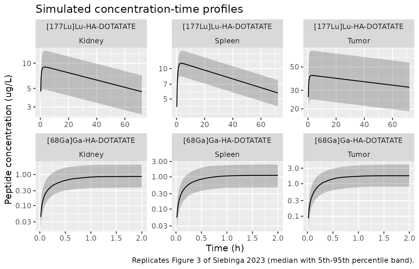
Figure 3 - concentration-time profiles in spleen, kidney and tumor
Figure 3 of Siebinga 2023 shows the individually observed decay-corrected peptide concentrations for both radiopharmaceuticals, stratified by patient. The panels below are the corresponding simulated population profiles (median with 5th-95th percentile band).
to_long <- function(sim, agent) {
  sim |>
    dplyr::select(id, time, Cspleen, Ckidney, Ctumor) |>
    tidyr::pivot_longer(
      c(Cspleen, Ckidney, Ctumor),
      names_to = "compartment", values_to = "conc"
    ) |>
    dplyr::mutate(
      agent = agent,
      compartment = dplyr::recode(compartment,
        Cspleen = "Spleen", Ckidney = "Kidney", Ctumor = "Tumor")
    )
}

prof <- dplyr::bind_rows(
  to_long(sim_ga, "[68Ga]Ga-HA-DOTATATE"),
  to_long(sim_lu, "[177Lu]Lu-HA-DOTATATE")
) |>
  dplyr::filter(time > 0) |>
  dplyr::group_by(agent, compartment, time) |>
  dplyr::summarise(
    Q05 = stats::quantile(conc, 0.05, na.rm = TRUE),
    Q50 = stats::quantile(conc, 0.50, na.rm = TRUE),
    Q95 = stats::quantile(conc, 0.95, na.rm = TRUE),
    .groups = "drop"
  )

ggplot(prof, aes(time, Q50)) +
  geom_ribbon(aes(ymin = Q05, ymax = Q95), alpha = 0.25) +
  geom_line() +
  facet_wrap(~agent + compartment, scales = "free", ncol = 3) +
  scale_y_log10() +
  labs(
    x = "Time (h)", y = "Peptide concentration (ug/L)",
    title = "Simulated concentration-time profiles",
    caption = "Replicates Figure 3 of Siebinga 2023 (median with 5th-95th percentile band)."
  )
Maximum receptor occupancy after
[177Lu]Lu-HA-DOTATATE
The Results section reports that maximum receptor occupancy after
[177Lu]Lu-HA-DOTATATE “ranged from 39 to 55% for spleen,
71-97% for kidney and 78-100% for tumors”. This is a direct,
quantitative check on the capacity-limited uptake mechanism, so it is
reproduced here from the typical-value profile of the median
patient.
mw <- 1628.5

typ <- tibble::tibble(
  id = 1L, TUM_VOL_TARGET = 80.0, TUM_VOL_TOTAL = 283
)
ev_typ <- dplyr::bind_rows(
  typ |> dplyr::mutate(time = 0, amt = 151, evid = 1L,
                       cmt = "blood", dvid = NA_integer_),
  typ |> tidyr::crossing(time = seq(0, 72, length.out = 1441)) |>
    dplyr::mutate(amt = NA_real_, evid = 0L, cmt = "tumor", dvid = 1L)
) |>
  dplyr::arrange(time, dplyr::desc(evid))

sim_typ <- rxode2::rxSolve(
  rxode2::zeroRe(mod_lu), ev_typ,
  useLinCmt = FALSE, returnType = "data.frame"
)
#> ℹ parameter labels from comments will be replaced by 'label()'
#> ℹ omega/sigma items treated as zero: 'etalkel', 'etalbmax_spleen', 'etalbmax_kidney', 'etalbmax_tumor', 'etalbmax_sstr'

# bmax as an amount (ug) = concentration (nmol/L) * mw/1000 * volume (L)
bmax_amt <- c(
  Spleen = 16.7 * mw / 1000 * 0.21,
  Kidney = 6.7 * mw / 1000 * 0.30,
  Tumor = 30.0 * mw / 1000 * (80.0 / 1000)
)

occupancy <- tibble::tibble(
  Compartment = c("Spleen", "Kidney", "Tumor"),
  `Simulated maximum occupancy (%)` = round(100 * c(
    max(sim_typ$spleen) / bmax_amt[["Spleen"]],
    max(sim_typ$kidney) / bmax_amt[["Kidney"]],
    max(sim_typ$tumor) / bmax_amt[["Tumor"]]
  ), 1),
  `Published range (%)` = c("39-55", "71-97", "78-100")
)

knitr::kable(
  occupancy,
  caption = "Maximum receptor occupancy after [177Lu]Lu-HA-DOTATATE, typical patient (target-lesion volume 80.0 mL, total tumor volume 283 mL, 151 ug peptide). Published values from Results, 'Semi-physiological PK model'."
)| Compartment | Simulated maximum occupancy (%) | Published range (%) |
|---|---|---|
| Spleen | 43.2 | 39-55 |
| Kidney | 84.8 | 71-97 |
| Tumor | 90.9 | 78-100 |
The paper’s contrasting statement for the diagnostic agent is that,
at the very low administered peptide amount, “receptors are not close to
full occupancy” – which is the stated rationale for placing
interindividual variability on the uptake rate constants for
[68Ga] but on the receptor expressions for
[177Lu].
ev_typ_ga <- dplyr::bind_rows(
  typ |> dplyr::mutate(time = 0, amt = 5.23, evid = 1L,
                       cmt = "blood", dvid = NA_integer_),
  typ |> tidyr::crossing(time = seq(0, 2, length.out = 241)) |>
    dplyr::mutate(amt = NA_real_, evid = 0L, cmt = "tumor", dvid = 1L)
) |>
  dplyr::arrange(time, dplyr::desc(evid))

sim_typ_ga <- rxode2::rxSolve(
  rxode2::zeroRe(mod_ga), ev_typ_ga,
  useLinCmt = FALSE, returnType = "data.frame"
)
#> ℹ parameter labels from comments will be replaced by 'label()'
#> ℹ omega/sigma items treated as zero: 'etalkel', 'etalkin_spleen', 'etalkin_kidney', 'etalkin_tumor', 'etalkin_sstr'
i45 <- which.min(abs(sim_typ_ga$time - 0.75))

tibble::tibble(
  Compartment = c("Spleen", "Kidney", "Tumor"),
  `Occupancy at the 45-min scan (%)` = round(100 * c(
    sim_typ_ga$spleen[i45] / bmax_amt[["Spleen"]],
    sim_typ_ga$kidney[i45] / bmax_amt[["Kidney"]],
    sim_typ_ga$tumor[i45] / bmax_amt[["Tumor"]]
  ), 1)
) |>
  knitr::kable(
    caption = "[68Ga]Ga-HA-DOTATATE receptor occupancy at the diagnostic scan time, typical patient (5.23 ug peptide). The paper states only that receptors are 'not close to full occupancy'."
)| Compartment | Occupancy at the 45-min scan (%) |
|---|---|
| Spleen | 3.5 |
| Kidney | 7.1 |
| Tumor | 3.0 |
PKNCA validation
Table 3 reports observed and model-predicted
AUC(0-tlast) for tumor and kidney after
[177Lu]Lu-HA-DOTATATE, with tlast = 72 h. One
PKNCA block is run per output compartment.
run_nca <- function(sim, conc_col, label) {
  sim_nca <- sim |>
    dplyr::mutate(Cc = .data[[conc_col]]) |>
    dplyr::filter(!is.na(Cc)) |>
    dplyr::mutate(compartment = label) |>
    dplyr::select(id, time, Cc, compartment)

  # Guarantee a time-zero row per subject so PKNCA can anchor AUC from 0.
  sim_nca <- dplyr::bind_rows(
    sim_nca,
    sim_nca |> dplyr::distinct(id, compartment) |>
      dplyr::mutate(time = 0, Cc = 0)
  ) |>
    dplyr::distinct(id, compartment, time, .keep_all = TRUE) |>
    dplyr::arrange(id, compartment, time)

  dose_df <- ev_lu |>
    dplyr::filter(evid == 1) |>
    dplyr::mutate(compartment = label) |>
    dplyr::select(id, time, amt, compartment)

  conc_obj <- PKNCA::PKNCAconc(sim_nca, Cc ~ time | compartment + id)
  dose_obj <- PKNCA::PKNCAdose(dose_df, amt ~ time | compartment + id)

  intervals <- data.frame(
    start = 0, end = 72,
    cmax = TRUE, tmax = TRUE, auclast = TRUE
  )

  PKNCA::pk.nca(PKNCA::PKNCAdata(conc_obj, dose_obj, intervals = intervals))
}

nca_tumor <- run_nca(sim_lu, "Ctumor", "Tumor")
nca_kidney <- run_nca(sim_lu, "Ckidney", "Kidney")
Comparison against published NCA
Table 3 reports AUC(0-tlast) in mgh/L; the simulated
auclast is in ugh/L, so it is divided by 1000 before
comparison. The reference values are the medians of the nine
observed patients in Table 3.
summarise_nca <- function(nca_res) {
  as.data.frame(nca_res$result) |>
    dplyr::filter(PPTESTCD %in% c("auclast", "cmax", "tmax")) |>
    dplyr::group_by(compartment, PPTESTCD) |>
    dplyr::summarise(value = stats::median(PPORRES, na.rm = TRUE), .groups = "drop") |>
    tidyr::pivot_wider(names_from = PPTESTCD, values_from = value) |>
    dplyr::mutate(auclast = auclast / 1000)  # ug*h/L -> mg*h/L
}

simulated <- dplyr::bind_rows(
  summarise_nca(nca_tumor),
  summarise_nca(nca_kidney)
)

# Table 3 observed AUC(0-tlast), mg*h/L:
#   tumor  3.32, 2.09, 5.29, 4.69, 1.38, 2.80, 2.94, 1.76, 2.59 -> median 2.80
#   kidney 0.520, 0.634, 0.334, 0.902, 0.564, 0.443, 0.764, 0.621 -> median 0.5925
published <- tibble::tribble(
  ~compartment, ~auclast,
  "Tumor",      2.80,
  "Kidney",     0.5925
)

cmp <- nlmixr2lib::ncaComparisonTable(
  simulated = simulated,
  reference = published,
  by = "compartment",
  params = "auclast",
  units = c(auclast = "mg*h/L"),
  tolerance_pct = 20
)

knitr::kable(
  cmp,
  caption = "Simulated vs. published [177Lu]Lu-HA-DOTATATE AUC(0-72 h). Reference = median of the nine observed patients in Table 3. * differs from reference by >20%."
)| NCA parameter | compartment | Reference | Simulated | % diff |
|---|---|---|---|---|
| AUClast (mg*h/L) | Tumor | 2.8 | 2.64 | -5.6% |
| AUClast (mg*h/L) | Kidney | 0.592 | 0.478 | -19.4% |
For context, the paper’s own model-predicted medians in Table 3 are 2.89 mgh/L (tumor) and 0.483 mgh/L (kidney), and the model-predicted kidney range (0.408-0.680) sits inside the wider observed range (0.334-0.902). The simulated population median for kidney is expected to land near the lower half of the observed range for the same reason the authors’ own predictions do: the kidney observations include urinary activity that the model does not represent, which is why the first (~1 h) kidney time point was excluded from parameter estimation altogether.
as.data.frame(nca_tumor$result) |>
  dplyr::bind_rows(as.data.frame(nca_kidney$result)) |>
  dplyr::filter(PPTESTCD == "auclast") |>
  dplyr::group_by(compartment) |>
  dplyr::summarise(
    `Median AUC(0-72 h) (mg*h/L)` = round(stats::median(PPORRES) / 1000, 3),
    `5th percentile` = round(stats::quantile(PPORRES, 0.05) / 1000, 3),
    `95th percentile` = round(stats::quantile(PPORRES, 0.95) / 1000, 3),
    .groups = "drop"
  ) |>
  dplyr::rename(Compartment = compartment) |>
  knitr::kable(
    caption = "Simulated [177Lu]Lu-HA-DOTATATE AUC(0-72 h) across the virtual cohort."
)| Compartment | Median AUC(0-72 h) (mg*h/L) | 5th percentile | 95th percentile |
|---|---|---|---|
| Kidney | 0.478 | 0.256 | 0.745 |
| Tumor | 2.643 | 1.563 | 4.526 |
Assumptions and deviations
Molar mass is not reported in this paper.
mw = 1628.5 g/molis inherited from the upstream framework paper this model is built on (Siebinga et al., EJNMMI Res. 2023;13:8, Table 3, “Molecular weight”), which is the sanctioned inherited-parameter path because the current paper explicitly fixes its structural parameters from that model. The constant is needed to reconcilebmax, reported in nmol/L, with the ug/L observation scale.Equation 4 is applied to spleen uptake only, exactly as printed. The surrounding prose describes the tumor sink effect as “a reduced uptake in healthy tissues” (plural), but the printed equation carries the effect on
k12alone. Per the standing trust-the-equation policy the equation is followed.Equation 4’s volume is in litres. The coefficient 0.4 multiplies a bare volume, so the unit is load-bearing and the paper does not state it. In litres the Table 1 range (22.4-644 mL) produces a 1-23% reduction in spleen uptake; in millilitres it would produce
exp(-113)and annihilate spleen uptake entirely. Litres is therefore the only self-consistent reading.The rest compartment’s uptake is un-gated but still restricted to the unbound fraction. Equation 1’s
bmaxterm is stated for the SSTR-expressing compartments (two to five), and Table 2 reports nobmaxfor compartment six, so no capacity gate is applied there.fuis applied, on the general prose statement that “only unbound molecules were available for uptake into compartments”. Both readings give a blood half-life in the tens of minutes and neither changes any of the validated quantities above.A single proportional residual error is replicated across three endpoints. Table 2 reports one 31.6% CV proportional error shared by every observed compartment. nlmixr2 requires a distinct endpoint parameter per observation channel, so
propSd_Cspleen,propSd_CkidneyandpropSd_Ctumorall carry the same published value; this is one estimate transcribed three times, not three independent estimates.Interindividual variability is fixed, not estimated, in both models. For the diagnostic model the paper says so explicitly (“IIV was fixed based on assumed population variability”); for the therapeutic model Table 2 reports the IIV terms without an RSE, and the table header states that RSEs are given for estimated values only.
Blood is predicted but never observed. No blood samples were drawn in this study, so
Ccis exposed as a prediction with no residual error model attached. The three observed channels are spleen, kidney and tumor.Virtual-cohort tumor volumes. Table 1 reports the target-lesion and total tumor volumes only as marginal medians and ranges, with no distributional family and no joint distribution. Target-lesion volume is drawn log-uniformly across the reported range (7.81-212 mL) so the reported extremes are honoured without inventing a shape, and total tumor volume is generated from the observed median ratio (283/80) with a 25% CV multiplicative scatter, clipped to its own reported range (22.4-644 mL). Only the marginal medians are anchored to published values; the spread and the correlation are assumptions of this vignette, not of the paper.
Cohort size. 120 virtual subjects per radiopharmaceutical, well under the 200-per-arm cap; the study itself had nine patients.
Supplement not used. Additional file 1 contains Figures S1-S3 (goodness-of-fit and individual-prediction plots) only, with no parameter content. No errata or corrigenda were found for this DOI.
Canonical names introduced with this extraction
This is the library’s first somatostatin-receptor radioligand model, and it introduced three canonical names, ratified by the maintainers:
-
sstr- the lumped somatostatin-receptor-expressing organ-group compartment (compartment five: lungs, pancreas, stomach, thyroid, liver), registered ininst/references/compartment-names.md. Distinct fromother, which is the non-receptor-expressing rest-of-body sink. -
TUM_VOL_TOTALandTUM_VOL_TARGET- clinical functional-imaging-segmented tumor volumes in mL, registered ininst/references/covariate-columns.md. Both are needed because they drive different effects with different coefficients, and only the target-lesion volume is the modelled compartment volume. Both are distinct from the preclinical caliperTUM_VOL(mm^3) and from the length-valuedTUMSZ/TUM_SLD.
The naming proposal also included a new
lkupt_<tissue> parameter family for the
capacity-limited uptake rate constant. Between the proposal being made
and ratified, the canonical lkin_<compartment> /
lkout_<compartment> tissue-exchange family was
registered in inst/references/parameter-names.md (founded
in part by this paper’s sibling model
Siebinga_2023_lu177psma617.R), and it covers precisely this
role. The register’s own precedence rule is to reuse an existing
canonical, so these models use lkin_<tissue> rather
than founding a duplicate name; the maintainers’ ratified intent – a
name distinct from the complex-internalisation kint
canonical, with suffixes drawn from the canonical compartment names – is
preserved. Likewise, bmax / lbmax had been
registered in the interim, so the ratified
bmax_<tissue> form is used as the already-sanctioned
site-suffixed variant rather than as a new entry.