Gepotidacin murine thigh-infection PK/PD (Singley 2026)
Source:vignettes/articles/Singley_2026_gepotidacin.Rmd
Singley_2026_gepotidacin.RmdModel and source
- Citation: Singley CM, Kurumaddali A, Hoover JL. Pharmacokinetic and pharmacodynamic characterization of gepotidacin against Escherichia coli and Klebsiella pneumoniae in a neutropenic mouse thigh infection model. Antimicrob Agents Chemother. 2026;70(1):e01176-25. doi:10.1128/aac.01176-25. Parameter values from Supplemental Material Table S1 and the Figure S1 equation.
- Article: Antimicrob Agents Chemother 2026;70(1):e01176-25
- Supplemental Material (Figures S1-S9, Tables S1-S7): https://doi.org/10.1128/aac.01176-25
Singley and colleagues characterised the pharmacokinetics and pharmacodynamics of gepotidacin, a first-in-class triazaacenaphthylene antibacterial, against 17 Escherichia coli and 7 Klebsiella pneumoniae isolates (gepotidacin MICs 0.25-16 ug/mL) in the neutropenic mouse thigh infection model. The free-drug fAUC/MIC target for a 1-log10 kill (13) supported the dose selection for uncomplicated urinary tract infection. The paper contributes:
- A population PK model
(
Singley_2026_gepotidacin): one compartment with first-order subcutaneous absorption, in which the absorption rate constant falls with the dose given at each administration. -
Twenty-six PK/PD models that couple the typical PK
to a three-parameter inhibitory Imax model of free-drug AUC0-24/MIC for
the change in thigh bacterial burden over the 24 h treatment period:
- two co-modelled fits pooling every isolate of a species
(
Singley_2026_gepotidacin_Ecoli_pooled, Figure S6;Singley_2026_gepotidacin_Kpneumoniae_pooled, Figure S7), and - twenty-four per-isolate fits, suffixed by species and isolate
(
Singley_2026_gepotidacin_Ecoli_ATCC25922, …,Singley_2026_gepotidacin_Kpneumoniae_1511289; Figures S8 and S9). The per-isolate fits are the ones from which the paper’s Table 2 targets are derived. Note thatSingley_2026_gepotidacin_Ecoli_ALLis the E. coli isolate designated “ALL” in Table 3, not a pooled fit.
- two co-modelled fits pooling every isolate of a species
(
Each fit has its own E0, Imax and IC50, so each is a separate file. Only the fAUC/MIC fits are packaged: the paper also fitted fAUC (not MIC-normalised), fCmax/MIC, %fT>MIC and four-parameter variants for index selection (Table S4), and concluded that “only fAUC/MIC was considered as the PK/PD index for further analyses”.
Population
Male CD-1 mice weighing 27-28 g were rendered neutropenic with
cyclophosphamide (150 mg/kg on day -4, 100 mg/kg on day -1) and infected
intramuscularly in one thigh; the inoculum was tailored per isolate to
give a baseline of about 6.5 log10 CFU per thigh 1 h after infection.
For PK, single subcutaneous doses of 6.25-800 mg/kg were given 1 h after
infection and plasma was taken by terminal cardiac puncture at 0.25,
0.5, 1, 2, 4 and 6 h (three mice per study, dose and time point;
HPLC-MS/MS, LLOQ 0.05 ug/mL). For PD, doses of 1-600 mg/kg were given
every 6 h for 24 h (four doses) starting 1 h after infection, with five
mice per group, and thighs were harvested at 25 h after infection.
Plasma protein binding in the mouse is 24% (concentration-independent).
The isolates and their MICs are listed in Table 3 of the paper; the
population metadata of each model records these facts, e.g.
readModelDb("Singley_2026_gepotidacin")()$population.
Source trace
| Equation / parameter | Value | Source location |
|---|---|---|
lka (Ka at 2.7 mg) |
0.886 /h | Table S1 ‘Kapop’ |
lcl (CL) |
0.101 L/h | Table S1 ‘CLpop’ |
lvc (V) |
0.018 L | Table S1 ‘Vpop’ |
e_dose_ka |
-0.437 | Table S1 ‘Dose effect on Kapop’; Figure S1 ‘Deff’ |
| Ka dose dependence | Ka = Kapop * (Dose/2.7)^Deff * exp(eta) |
Figure S1 equation |
etalcl |
38.9% CV | Table S1 ‘IIV on CL’ |
etalka |
20.3% CV (variance 0.04) | Table S1 ‘IIV on Ka’; Figure S1 |
addSd |
0.128 mg/L | Table S1 ‘Add err’ |
| Inhibitory Imax model |
E = E0 - Imax * X / (IC50 + X), X = fAUC0-24/MIC |
Figure S5; Table S4 footnote (gamma = 1) |
pooled e0, limax, lic50
|
per species | Figures S6 and S7 parameter tables |
per-isolate e0, limax,
lic50
|
per isolate | Figures S8 and S9 per-panel tables |
mic per isolate |
0.25-16 ug/mL | Table 3; Figures S8 and S9 |
mic default of the pooled fits |
MIC90 4 (E. coli), 16 (K. pneumoniae) ug/mL | Materials and Methods ‘Bacterial isolates’ |
log10_cfu0 |
6.5 log10 CFU | Materials and Methods ‘Infection’ |
| stasis / 1-log / 2-log targets | per isolate | Table 2, Tables S5-S7, Figures S6-S9 |
The E0, Imax and IC50 values are printed in the tables beneath each plot panel of Figures S6-S9 in the Supplemental Material and were transcribed from them.
PK simulation
The dose amount is in mg per mouse. Doses in mg/kg are converted with
a 27 g body weight, the weight at which the model’s 2.7 mg reference
dose equals the central 100 mg/kg dose. DOSE (the dose per
administration, a model covariate) must be supplied on every record,
after the event columns.
bw_kg <- 0.027
pk <- rxode2::rxode(readModelDb("Singley_2026_gepotidacin"))
#> ℹ parameter labels from comments will be replaced by 'label()'

# One subject per dose level, so dose levels stay distinct subjects.
make_events <- function(dose_mgkg, times, n_doses = 1, id = 1) {
  dose_mg <- dose_mgkg * bw_kg
  dplyr::bind_rows(
    tibble(id = id, time = 6 * (seq_len(n_doses) - 1), amt = dose_mg, evid = 1, cmt = "depot"),
    tibble(id = id, time = times, amt = NA_real_, evid = 0, cmt = "central")
  ) |>
    dplyr::arrange(time, dplyr::desc(evid)) |>
    dplyr::mutate(DOSE = dose_mg, dose_mgkg = dose_mgkg)
}
sd_doses <- c(6.25, 50, 100, 200, 400, 800)
sd_times <- sort(unique(c(seq(0, 6, by = 0.05), 0.25, 0.5, 1, 2, 4, 6)))
ev_sd <- dplyr::bind_rows(lapply(seq_along(sd_doses), function(i) {
  make_events(sd_doses[i], sd_times, id = i)
}))
sim_sd <- rxode2::rxSolve(rxode2::zeroRe(pk), events = ev_sd, keep = "dose_mgkg") |>
  as.data.frame()
#> ℹ omega/sigma items treated as zero: 'etalcl', 'etalka'
#> Warning: multi-subject simulation without without 'omega'

# Concentrations below 0.01 ug/mL fall outside the plotted range.
ggplot(dplyr::filter(sim_sd, Cc >= 0.01), aes(time, Cc, colour = factor(dose_mgkg))) +
  geom_line() +
  geom_hline(yintercept = 0.05, linetype = "dashed") +
  scale_y_log10(limits = c(0.01, 100)) +
  labs(
    x = "Time after dose (h)", y = "Free gepotidacin (ug/mL)", colour = "Dose (mg/kg)",
    title = "Typical free plasma gepotidacin after a single subcutaneous dose",
    caption = "Dashed line: LLOQ 0.05 ug/mL."
  )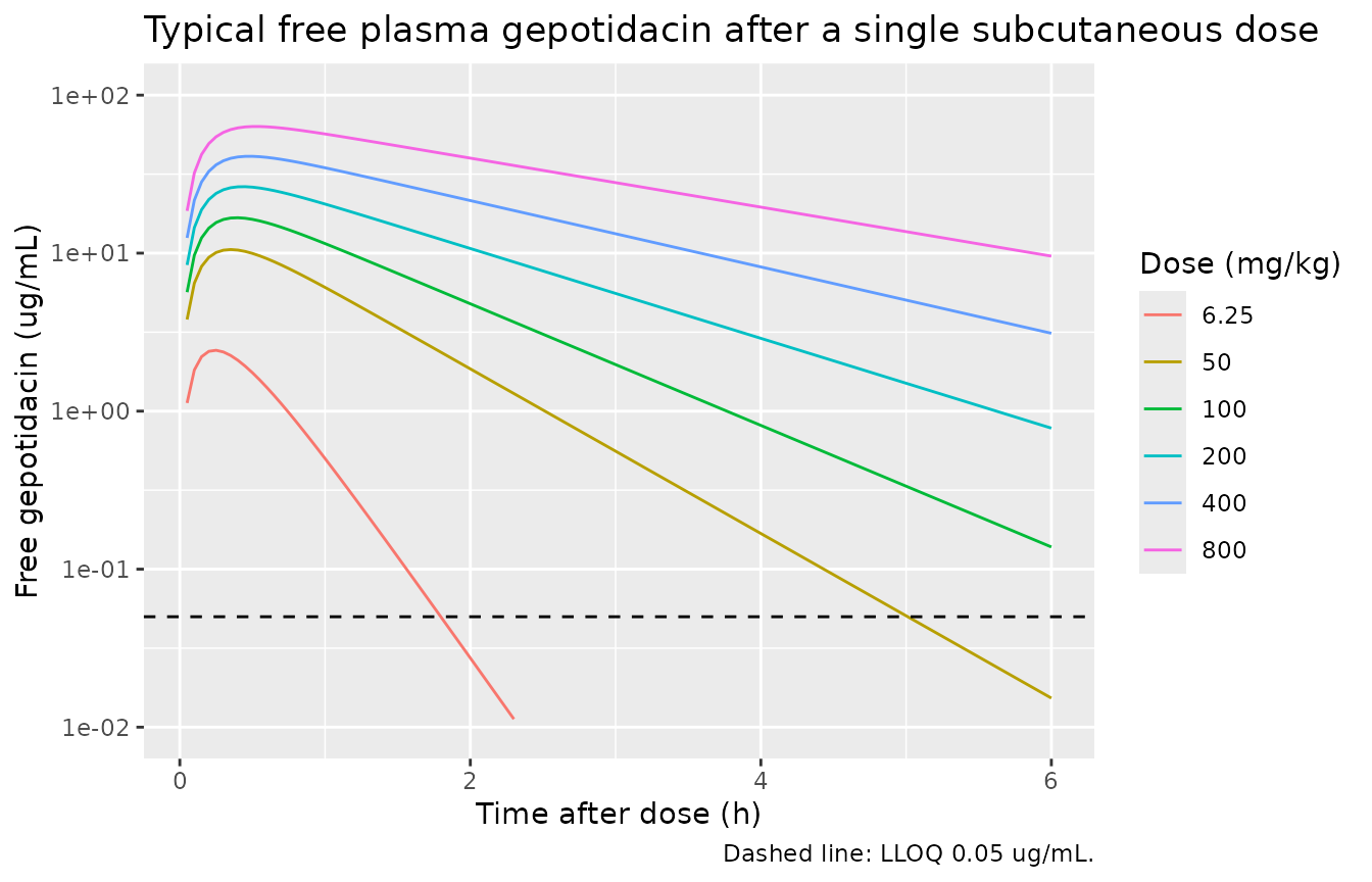
Replicates Figure 1 of Singley 2026.
A stochastic cohort sampled at the paper’s design (terminal sampling, so each time point is a different mouse) gives the mean and standard deviation that Figure 1 plots. A modest cohort per dose is enough for the envelope.
rxode2::rxSetSeed(20261)
obs_times <- c(0.25, 0.5, 1, 2, 4, 6)
n_per_time <- 30
ev_vpc <- dplyr::bind_rows(lapply(seq_along(sd_doses), function(i) {
  dplyr::bind_rows(lapply(seq_along(obs_times), function(j) {
    dplyr::bind_rows(lapply(seq_len(n_per_time), function(k) {
      make_events(sd_doses[i], obs_times[j],
        id = ((i - 1) * length(obs_times) + (j - 1)) * n_per_time + k
      )
    }))
  }))
}))
sim_vpc <- rxode2::rxSolve(pk, events = ev_vpc, keep = "dose_mgkg") |>
  as.data.frame()

vpc_sum <- sim_vpc |>
  dplyr::group_by(dose_mgkg, time) |>
  dplyr::summarise(mean = mean(sim), sd = sd(sim), .groups = "drop")

ggplot(vpc_sum, aes(time, mean, colour = factor(dose_mgkg))) +
  geom_errorbar(aes(ymin = mean - sd, ymax = mean + sd), width = 0.1) +
  geom_point() +
  geom_line() +
  labs(
    x = "Time after dose (h)", y = "Free gepotidacin (ug/mL)", colour = "Dose (mg/kg)",
    title = "Simulated terminal-sampling composite profiles"
  )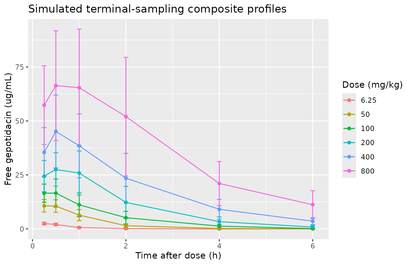
Mean +- SD of a simulated terminal-sampling cohort; compare Figure 1 of Singley 2026.
NCA validation
Repeat dosing: Table S2
Table S2 reports fAUC0-24 and fCmax computed by the authors from simulations of the final PK model for the every-6-h dose-ranging regimens of the efficacy studies. Both sides come from the same model, so this is a tight check of the transcription.
s2_doses <- c(1, 6.25, 12.5, 25, 50, 100, 200, 400, 600)
ev_s2 <- dplyr::bind_rows(lapply(seq_along(s2_doses), function(i) {
  make_events(s2_doses[i], seq(0, 24, by = 0.01), n_doses = 4, id = i)
}))
sim_s2 <- rxode2::rxSolve(rxode2::zeroRe(pk), events = ev_s2, keep = "dose_mgkg") |>
  as.data.frame()
#> ℹ omega/sigma items treated as zero: 'etalcl', 'etalka'
#> Warning: multi-subject simulation without without 'omega'

conc_s2 <- sim_s2 |>
  dplyr::filter(!is.na(Cc)) |>
  dplyr::mutate(treatment = as.character(dose_mgkg)) |>
  dplyr::select(id, time, Cc, treatment)
conc_s2 <- dplyr::bind_rows(
  conc_s2,
  conc_s2 |> dplyr::distinct(id, treatment) |> dplyr::mutate(time = 0, Cc = 0)
) |>
  dplyr::distinct(id, treatment, time, .keep_all = TRUE) |>
  dplyr::arrange(id, time)
dose_s2 <- ev_s2 |>
  dplyr::filter(evid == 1) |>
  dplyr::mutate(treatment = as.character(dose_mgkg)) |>
  dplyr::select(id, time, amt, treatment)

nca_s2 <- PKNCA::pk.nca(PKNCA::PKNCAdata(
  PKNCA::PKNCAconc(conc_s2, Cc ~ time | treatment + id),
  PKNCA::PKNCAdose(dose_s2, amt ~ time | treatment + id),
  intervals = data.frame(start = 0, end = 24, cmax = TRUE, auclast = TRUE)
))

published_s2 <- tibble::tribble(
  ~treatment, ~auclast, ~cmax,
  "1",        0.87,     0.56,
  "6.25",     6.20,     2.49,
  "12.5",     12.78,    4.10,
  "25",       26.13,    6.58,
  "50",       53.09,    10.34,
  "100",      107.28,   16.88,
  "200",      215.41,   27.42,
  "400",      428.79,   44.73,
  "600",      638.08,   60.04
)

nlmixr2lib::ncaComparisonTable(
  simulated = nca_s2,
  reference = published_s2,
  by = "treatment",
  units = c(cmax = "ug/mL", auclast = "ug*h/mL")
) |>
  dplyr::rename("Dose (mg/kg q6h)" = treatment) |>
  knitr::kable(
    caption = "Simulated typical-value fAUC0-24 and fCmax versus Table S2. * differs by more than 20%.",
    digits = 2
)| NCA parameter | Dose (mg/kg q6h) | Reference | Simulated | % diff |
|---|---|---|---|---|
| Cmax (ug/mL) | 1 | 0.56 | 0.598 | +6.8% |
| Cmax (ug/mL) | 6.25 | 2.49 | 2.43 | -2.4% |
| Cmax (ug/mL) | 12.5 | 4.1 | 4.02 | -2.0% |
| Cmax (ug/mL) | 25 | 6.58 | 6.55 | -0.5% |
| Cmax (ug/mL) | 50 | 10.3 | 10.5 | +2.0% |
| Cmax (ug/mL) | 100 | 16.9 | 16.9 | -0.2% |
| Cmax (ug/mL) | 200 | 27.4 | 26.9 | -1.7% |
| Cmax (ug/mL) | 400 | 44.7 | 43.6 | -2.4% |
| Cmax (ug/mL) | 600 | 60 | 58.5 | -2.6% |
| AUClast (ug*h/mL) | 1 | 0.87 | 1.07 | +22.9%* |
| AUClast (ug*h/mL) | 6.25 | 6.2 | 6.68 | +7.8% |
| AUClast (ug*h/mL) | 12.5 | 12.8 | 13.4 | +4.6% |
| AUClast (ug*h/mL) | 25 | 26.1 | 26.7 | +2.3% |
| AUClast (ug*h/mL) | 50 | 53.1 | 53.4 | +0.7% |
| AUClast (ug*h/mL) | 100 | 107 | 107 | -0.5% |
| AUClast (ug*h/mL) | 200 | 215 | 213 | -1.3% |
| AUClast (ug*h/mL) | 400 | 429 | 421 | -1.8% |
| AUClast (ug*h/mL) | 600 | 638 | 625 | -2.1% |
s2_chk <- as.data.frame(nca_s2$result) |>
  dplyr::filter(PPTESTCD %in% c("auclast", "cmax")) |>
  dplyr::select(treatment, PPTESTCD, PPORRES) |>
  dplyr::left_join(
    tidyr::pivot_longer(published_s2, -treatment, names_to = "PPTESTCD", values_to = "ref"),
    by = c("treatment", "PPTESTCD")
  ) |>
  dplyr::mutate(pct = 100 * (PPORRES / ref - 1), dose = as.numeric(treatment))
# Typical-value model against the authors' own simulations: deterministic on
# both sides, so a tight bound holds from 12.5 mg/kg up.
stopifnot(all(abs(s2_chk$pct[s2_chk$dose >= 12.5]) < 5))
From 25 mg/kg up, fAUC0-24 and fCmax agree with Table S2 to within 3% (5% at 12.5 mg/kg), which confirms both the dose unit (mg per mouse, 27 g mouse) and that the model predicts free rather than total concentrations: scaling by the 0.76 unbound fraction would put every row about 24% low. At the two lowest doses the simulated fAUC0-24 is 8% (6.25 mg/kg) and 23% (1 mg/kg) above Table S2 while fCmax agrees within 7%. Censoring concentrations below the 0.05 ug/mL LLOQ before integrating does not close that gap (it gives 1.03 ug*h/mL at 1 mg/kg), nor does integrating only at the PK sampling times; how the authors’ R NCA treated the low-concentration tail is not described.
%fT>MIC: Table S3
published_s3 <- tibble::tribble(
  ~dose, ~`0.25`, ~`0.5`, ~`1`, ~`2`, ~`4`, ~`8`, ~`16`,
  1,      7.7,     3.3,    0.0,  0.0,  0.0,  0.0,  0.0,
  6.25,   20.8,    16.7,   11.7, 5.3,  0.0,  0.0,  0.0,
  12.5,   29.7,    24.2,   18.5, 12.3, 2.2,  0.0,  0.0,
  25,     42.8,    35.5,   28.2, 20.5, 12.2, 0.0,  0.0,
  50,     62.2,    52.3,   42.3, 32.5, 22.2, 10.5, 0.0,
  100,    90.5,    77.2,   64.0, 50.5, 37.0, 23.0, 5.8,
  200,    100,     100,    95.9, 77.8, 59.8, 41.4, 22.3,
  400,    100,     100,    100,  100,  94.7, 70.2, 45.4,
  600,    100,     100,    100,  100,  99.9, 94.1, 64.8
) |>
  tidyr::pivot_longer(-dose, names_to = "mic", values_to = "published") |>
  dplyr::mutate(mic = as.numeric(mic))

ftmic <- sim_s2 |>
  dplyr::filter(time < 24) |>
  tidyr::crossing(mic = unique(published_s3$mic)) |>
  dplyr::group_by(dose = dose_mgkg, mic) |>
  dplyr::summarise(simulated = 100 * mean(Cc > mic), .groups = "drop") |>
  dplyr::left_join(published_s3, by = c("dose", "mic")) |>
  dplyr::mutate(diff = simulated - published)

ftmic |>
  dplyr::select(dose, mic, simulated) |>
  tidyr::pivot_wider(names_from = mic, values_from = simulated) |>
  dplyr::rename("Dose (mg/kg q6h)" = dose) |>
  knitr::kable(
    caption = "Simulated typical-value %fT>MIC over 0-24 h by MIC (ug/mL); compare Table S3.",
    digits = 1
)| Dose (mg/kg q6h) | 0.25 | 0.5 | 1 | 2 | 4 | 8 | 16 |
|---|---|---|---|---|---|---|---|
| 1.0 | 7.5 | 3.3 | 0.0 | 0.0 | 0.0 | 0.0 | 0.0 |
| 6.2 | 20.7 | 16.5 | 11.7 | 5.2 | 0.0 | 0.0 | 0.0 |
| 12.5 | 29.3 | 23.8 | 18.3 | 12.0 | 1.0 | 0.0 | 0.0 |
| 25.0 | 42.2 | 35.0 | 27.7 | 20.2 | 11.7 | 0.0 | 0.0 |
| 50.0 | 61.1 | 51.5 | 41.7 | 31.8 | 21.7 | 10.0 | 0.0 |
| 100.0 | 88.8 | 75.8 | 62.8 | 49.5 | 36.2 | 22.5 | 4.8 |
| 200.0 | 100.0 | 100.0 | 94.0 | 76.3 | 58.5 | 40.4 | 21.7 |
| 400.0 | 100.0 | 100.0 | 100.0 | 100.0 | 92.6 | 68.5 | 44.0 |
| 600.0 | 100.0 | 100.0 | 100.0 | 100.0 | 99.9 | 91.9 | 63.0 |
# Same model on both sides; the residual is the time grid and the authors'
# rounding, so the bound is in percentage points of the 24 h interval.
stopifnot(quantile(abs(ftmic$diff), 0.9) < 5)
The largest difference from Table S3 is 2.2 percentage points of the dosing day.
Single dose: Table 1
Table 1 is non-compartmental analysis of the observed composite profiles (the mean of three mice per time point, pooled over studies), so it measures how well the model fits the data rather than the transcription. The typical-value model, sampled at the PK design times, is compared below.
conc_t1 <- sim_sd |>
  dplyr::filter(time %in% c(0, obs_times)) |>
  dplyr::mutate(treatment = as.character(dose_mgkg)) |>
  dplyr::select(id, time, Cc, treatment)
dose_t1 <- ev_sd |>
  dplyr::filter(evid == 1) |>
  dplyr::mutate(treatment = as.character(dose_mgkg)) |>
  dplyr::select(id, time, amt, treatment)

nca_t1 <- PKNCA::pk.nca(PKNCA::PKNCAdata(
  PKNCA::PKNCAconc(conc_t1, Cc ~ time | treatment + id),
  PKNCA::PKNCAdose(dose_t1, amt ~ time | treatment + id),
  intervals = data.frame(start = 0, end = 6, cmax = TRUE, auclast = TRUE),
  options = list(auc.method = "linear")
))

published_t1 <- tibble::tribble(
  ~treatment, ~cmax, ~auclast,
  "6.25",     1.21,  1.27,
  "50",       9.04,  8.58,
  "100",      18.5,  30.7,
  "200",      26.9,  46.2,
  "400",      42.7,  124,
  "800",      75.1,  260
)

nlmixr2lib::ncaComparisonTable(
  simulated = nca_t1,
  reference = published_t1,
  by = "treatment",
  units = c(cmax = "ug/mL", auclast = "ug*h/mL")
) |>
  dplyr::rename("Dose (mg/kg)" = treatment) |>
  knitr::kable(
    caption = paste(
      "Typical-value fCmax and fAUC0-6 at the sampling times versus the observed",
      "composite NCA of Table 1. * differs by more than 20%."
    ),
    digits = 2
)| NCA parameter | Dose (mg/kg) | Reference | Simulated | % diff |
|---|---|---|---|---|
| Cmax (ug/mL) | 6.25 | 1.21 | 2.43 | +100.6%* |
| Cmax (ug/mL) | 50 | 9.04 | 10.1 | +11.7% |
| Cmax (ug/mL) | 100 | 18.5 | 16.4 | -11.6% |
| Cmax (ug/mL) | 200 | 26.9 | 26.2 | -2.7% |
| Cmax (ug/mL) | 400 | 42.7 | 41 | -4.0% |
| Cmax (ug/mL) | 800 | 75.1 | 63.3 | -15.7% |
| AUClast (ug*h/mL) | 6.25 | 1.27 | 1.68 | +32.3%* |
| AUClast (ug*h/mL) | 50 | 8.58 | 13.9 | +62.5%* |
| AUClast (ug*h/mL) | 100 | 30.7 | 27.6 | -10.1% |
| AUClast (ug*h/mL) | 200 | 46.2 | 53.7 | +16.3% |
| AUClast (ug*h/mL) | 400 | 124 | 102 | -17.6% |
| AUClast (ug*h/mL) | 800 | 260 | 189 | -27.5%* |
t1_chk <- as.data.frame(nca_t1$result) |>
  dplyr::filter(PPTESTCD %in% c("auclast", "cmax")) |>
  dplyr::left_join(
    tidyr::pivot_longer(published_t1, -treatment, names_to = "PPTESTCD", values_to = "ref"),
    by = c("treatment", "PPTESTCD")
  ) |>
  dplyr::mutate(pct = 100 * (PPORRES / ref - 1))
# Model against observed data: a mis-transcribed clearance, volume or dose unit
# would shift the whole set by tens of percent.
stopifnot(abs(median(t1_chk$pct)) < 15)
From 50 to 800 mg/kg, fCmax agrees with Table 1 to within 16%. At 6.25 mg/kg the model predicts twice the observed peak (2.43 versus 1.21 ug/mL); the authors’ own simulations give the same value (Table S2: fCmax 2.49 ug/mL for 6.25 mg/kg every 6 h, a regimen with negligible accumulation), so it is a property of the published model, whose dose effect makes absorption fast at low doses, and not of the transcription. fAUC0-6 is the noisier comparison because the observed composite profiles are not smooth in dose: the observed fAUC0-6 at 50 mg/kg (8.58 ug*h/mL) is below its own fCmax of 9.04 ug/mL, and the model over-predicts it by about 60%; at 400 and 800 mg/kg the observed fAUC0-6 rises more steeply than the model follows (-18% and -28%), matching the upward trend at high predictions in the NPDE-versus-prediction diagnostic of Figure S4. Across the twelve comparisons the median difference is -3.4%.
PK/PD models
Reproducing the published fAUC/MIC targets
With the Hill coefficient fixed at 1, the fAUC/MIC giving an effect E
is X = (E0 - E) * IC50 / (Imax - E0 + E). Evaluating that
at E = 0, -1 and -2 for every packaged model reproduces the stasis,
1-log10 and 2-log10 kill targets printed beneath Figures S6-S9 and in
Tables 2, S5 and S6.
pd_names <- c(
  "Singley_2026_gepotidacin_Ecoli_pooled", "Singley_2026_gepotidacin_Kpneumoniae_pooled",
  paste0("Singley_2026_gepotidacin_Ecoli_", c(
    "Y6702902277A", "Y6702665868B", "Y6700050509B", "Y6700034261B", "ATCC25922",
    "NCTC13441", "997577", "ALL", "IR5", "1139570", "774319", "817317", "771034",
    "764023", "1032890", "823196", "718513"
  )),
  paste0("Singley_2026_gepotidacin_Kpneumoniae_", c(
    "1286210", "1478575", "1478677", "1203214", "1449616", "1511191", "1511289"
  ))
)

# Published targets and the mean growth of vehicle-treated controls. The two
# isolates whose E0 is negative have a negative stasis solution, printed as
# '0 (-1.2)' and '0 (-1.7)'; the negative solution is compared here and 0 is
# used in the summary statistics, as in Tables S5 and S6.
published_targets <- tibble::tribble(
  ~isolate,       ~stasis, ~kill1, ~kill2, ~vtc,
  "pooled_Ecoli", 5.1,     11.5,   22.4,   NA,
  "pooled_Kpneumoniae", 3.6, 7.3,  13.5,   NA,
  "Y6702902277A", 0.6,     1.4,    2.9,    1.26,
  "Y6702665868B", 7.7,     18.3,   37.9,   2.04,
  "Y6700050509B", 1.5,     3.2,    5.9,    1.38,
  "Y6700034261B", 2.8,     8.1,    17.1,   0.65,
  "ATCC25922",    13.7,    23.1,   37.7,   2.27,
  "NCTC13441",    17.1,    28.3,   47.2,   2.89,
  "997577",       10.5,    18.4,   32.5,   2.48,
  "ALL",          2.9,     6.7,    14.8,   1.52,
  "IR5",          2.5,     4.9,    10.2,   2.05,
  "1139570",      2,       4.8,    9.8,    1.28,
  "774319",       4.6,     16.1,   31.8,   0.32,
  "817317",       0.1,     0.8,    2.1,    0.35,
  "771034",       22.6,    37.2,   63,     3.30,
  "764023",       1.2,     2.2,    4.4,    2.96,
  "1032890",      21.4,    29.9,   39.5,   2.94,
  "823196",       0.4,     2.6,    6.9,    0.33,
  "718513",       -1.2,    2.3,    12.6,   -0.38,
  "1286210",      -1.7,    3.9,    12.4,   -0.33,
  "1478575",      5.3,     10.4,   20.6,   2.06,
  "1478677",      3.1,     5.7,    10.1,   1.73,
  "1203214",      5.6,     10.4,   19.4,   2.37,
  "1449616",      2,       5.6,    11.6,   1.21,
  "1511191",      1.1,     2.8,    6.6,    1.26,
  "1511289",      5.9,     9.5,     15.6,  3.22
)

pd_par <- dplyr::bind_rows(lapply(pd_names, function(mn) {
  th <- rxode2::rxode(readModelDb(mn))$theta
  rest <- sub("^Singley_2026_gepotidacin_", "", mn)
  species <- sub("_.*$", "", rest)
  isolate <- sub("^[^_]+_", "", rest)
  tibble(
    model = mn, species = species,
    isolate = ifelse(isolate == "pooled", paste0("pooled_", species), isolate),
    e0 = th[["e0"]], imax = exp(th[["limax"]]), ic50 = exp(th[["lic50"]]), mic = th[["mic"]]
  )
}))

target_x <- function(e0, imax, ic50, effect) (e0 - effect) * ic50 / (imax - e0 + effect)

tgt <- pd_par |>
  dplyr::mutate(
    stasis_model = target_x(e0, imax, ic50, 0),
    kill1_model = target_x(e0, imax, ic50, -1),
    kill2_model = target_x(e0, imax, ic50, -2)
  ) |>
  dplyr::left_join(published_targets, by = "isolate")

tgt |>
  dplyr::select(isolate, mic, e0, imax, ic50, stasis_model, stasis, kill1_model, kill1, kill2_model, kill2) |>
  dplyr::rename(
    "Isolate" = isolate, "MIC" = mic, "E0" = e0, "Imax" = imax, "IC50" = ic50,
    "Stasis (model)" = stasis_model, "Stasis (paper)" = stasis,
    "1-log (model)" = kill1_model, "1-log (paper)" = kill1,
    "2-log (model)" = kill2_model, "2-log (paper)" = kill2
  ) |>
knitr::kable(digits = 2, caption = "fAUC/MIC targets from the packaged parameters versus the published targets.")| Isolate | MIC | E0 | Imax | IC50 | Stasis (model) | Stasis (paper) | 1-log (model) | 1-log (paper) | 2-log (model) | 2-log (paper) |
|---|---|---|---|---|---|---|---|---|---|---|
| pooled_Ecoli | 4.00 | 1.33 | 6.03 | 18.15 | 5.14 | 5.1 | 11.43 | 11.5 | 22.38 | 22.4 |
| pooled_Kpneumoniae | 16.00 | 1.71 | 6.54 | 10.24 | 3.63 | 3.6 | 7.25 | 7.3 | 13.42 | 13.5 |
| Y6702902277A | 0.25 | 1.30 | 5.70 | 2.20 | 0.65 | 0.6 | 1.49 | 1.4 | 3.02 | 2.9 |
| Y6702665868B | 0.25 | 1.20 | 5.60 | 28.20 | 7.69 | 7.7 | 18.25 | 18.3 | 37.60 | 37.9 |
| Y6700050509B | 0.50 | 1.30 | 6.80 | 6.40 | 1.51 | 1.5 | 3.27 | 3.2 | 6.03 | 5.9 |
| Y6700034261B | 0.50 | 0.80 | 5.70 | 18.10 | 2.96 | 2.8 | 8.35 | 8.1 | 17.48 | 17.1 |
| ATCC25922 | 1.00 | 2.60 | 8.20 | 29.00 | 13.46 | 13.7 | 22.70 | 23.1 | 37.06 | 37.7 |
| NCTC13441 | 2.00 | 3.10 | 8.00 | 27.20 | 17.21 | 17.1 | 28.59 | 28.3 | 47.83 | 47.2 |
| 997577 | 2.00 | 2.70 | 7.20 | 17.70 | 10.62 | 10.5 | 18.71 | 18.4 | 33.28 | 32.5 |
| ALL | 4.00 | 1.50 | 5.20 | 7.30 | 2.96 | 2.9 | 6.76 | 6.7 | 15.03 | 14.8 |
| IR5 | 4.00 | 2.10 | 5.90 | 4.40 | 2.43 | 2.5 | 4.87 | 4.9 | 10.02 | 10.2 |
| 1139570 | 8.00 | 1.10 | 5.70 | 7.90 | 1.89 | 2.0 | 4.61 | 4.8 | 9.42 | 9.8 |
| 774319 | 8.00 | 0.50 | 7.90 | 69.00 | 4.66 | 4.6 | 16.17 | 16.1 | 31.94 | 31.8 |
| 817317 | 8.00 | 0.20 | 4.40 | 2.00 | 0.10 | 0.1 | 0.75 | 0.8 | 2.00 | 2.1 |
| 771034 | 8.00 | 3.50 | 8.10 | 29.70 | 22.60 | 22.6 | 37.12 | 37.2 | 62.83 | 63.0 |
| 764023 | 16.00 | 3.10 | 6.70 | 1.40 | 1.21 | 1.2 | 2.21 | 2.2 | 4.46 | 4.4 |
| 1032890 | 16.00 | 3.20 | 19.90 | 111.70 | 21.40 | 21.4 | 29.88 | 29.9 | 39.51 | 39.5 |
| 823196 | 16.00 | 0.25 | 4.40 | 6.60 | 0.40 | 0.4 | 2.62 | 2.6 | 6.91 | 6.9 |
| 718513 | 16.00 | -0.40 | 2.60 | 8.20 | -1.09 | -1.2 | 2.46 | 2.3 | 13.12 | 12.6 |
| 1286210 | 2.00 | -0.34 | 5.62 | 29.67 | -1.69 | -1.7 | 3.95 | 3.9 | 12.44 | 12.4 |
| 1478575 | 4.00 | 2.23 | 6.16 | 9.45 | 5.36 | 5.3 | 10.42 | 10.4 | 20.71 | 20.6 |
| 1478677 | 4.00 | 2.03 | 7.18 | 7.85 | 3.09 | 3.1 | 5.73 | 5.7 | 10.04 | 10.1 |
| 1203214 | 8.00 | 2.27 | 6.64 | 10.74 | 5.58 | 5.6 | 10.42 | 10.4 | 19.35 | 19.4 |
| 1449616 | 8.00 | 0.78 | 5.79 | 12.60 | 1.96 | 2.0 | 5.59 | 5.6 | 11.64 | 11.6 |
| 1511191 | 16.00 | 1.09 | 4.74 | 3.54 | 1.06 | 1.1 | 2.79 | 2.8 | 6.63 | 6.6 |
| 1511289 | 16.00 | 3.55 | 8.47 | 8.20 | 5.92 | 5.9 | 9.52 | 9.5 | 15.59 | 15.6 |
tgt_long <- dplyr::bind_rows(
  dplyr::transmute(tgt, isolate, endpoint = "stasis", model = stasis_model, paper = stasis),
  dplyr::transmute(tgt, isolate, endpoint = "kill1", model = kill1_model, paper = kill1),
  dplyr::transmute(tgt, isolate, endpoint = "kill2", model = kill2_model, paper = kill2)
) |>
  dplyr::mutate(pct = 100 * (model / paper - 1))
# The E0, Imax and IC50 under each panel are printed to two or three
# significant figures while the targets were computed from unrounded values, so
# small targets carry a few percent of rounding error. A mis-read digit moves a
# target by tens of percent.
stopifnot(
  abs(median(tgt_long$pct)) < 3,
  quantile(abs(tgt_long$pct), 0.9) < 10
)
Across all 78 targets the median difference is 0.2% and 90% are within 4.8%; the remaining differences are rounding of the printed parameters (for example E. coli Y6702902277A, whose IC50 is printed as 2.2).
Reproducing the Table 2 and Tables S5-S7 summary statistics
The paper’s headline target is the median 1-log10-kill fAUC/MIC over the E. coli isolates that grew at least 1 log10 in vehicle-treated controls: 13. The same medians computed from the packaged per-isolate models:
iso <- tgt |>
  dplyr::filter(!grepl("^pooled", isolate)) |>
  dplyr::mutate(
    stasis_model = pmax(stasis_model, 0),
    grew = vtc >= 1,
    # Tables S5-S7 'Summary using 1-log10 reduction endpoint for isolates with
    # >= 1 log10 of growth and 2-log10 reduction endpoint for isolates with <1
    # log10 of growth'.
    mixed_model = ifelse(grew, kill1_model, kill2_model)
  )
summ <- function(d, label) {
  tibble(
    group = label,
    `Stasis (growers)` = median(d$stasis_model[d$grew]),
    `1-log (growers)` = median(d$kill1_model[d$grew]),
    `2-log (growers)` = median(d$kill2_model[d$grew]),
    `1-log (all)` = median(d$kill1_model),
    `Mixed endpoint (all)` = median(d$mixed_model)
  )
}
summary_model <- dplyr::bind_rows(
  summ(dplyr::filter(iso, species == "Ecoli"), "E. coli"),
  summ(dplyr::filter(iso, species == "Kpneumoniae"), "K. pneumoniae"),
  summ(iso, "All isolates")
)
summary_paper <- tibble::tribble(
  ~group,          ~`Stasis (growers)`, ~`1-log (growers)`, ~`2-log (growers)`, ~`1-log (all)`, ~`Mixed endpoint (all)`,
  "E. coli",       5.3,                 13,                 24,                 6.7,            13,
  "K. pneumoniae", 4.2,                 7.6,                14,                 5.7,            9.5,
  "All isolates",  4.2,                 8.1,                15,                 6.2,            10
)
dplyr::bind_rows(
  dplyr::mutate(summary_model, source = "Packaged models"),
  dplyr::mutate(summary_paper, source = "Table 2 / Tables S5-S7")
) |>
  dplyr::arrange(group, source) |>
  dplyr::rename("Group" = group, "Source" = source) |>
knitr::kable(digits = 1, caption = "Median fAUC/MIC targets.")| Group | Stasis (growers) | 1-log (growers) | 2-log (growers) | 1-log (all) | Mixed endpoint (all) | Source |
|---|---|---|---|---|---|---|
| All isolates | 4.2 | 8.1 | 15.3 | 6.2 | 10.0 | Packaged models |
| All isolates | 4.2 | 8.1 | 15.0 | 6.2 | 10.0 | Table 2 / Tables S5-S7 |
| E. coli | 5.3 | 12.5 | 24.2 | 6.8 | 13.1 | Packaged models |
| E. coli | 5.3 | 13.0 | 24.0 | 6.7 | 13.0 | Table 2 / Tables S5-S7 |
| K. pneumoniae | 4.2 | 7.6 | 13.6 | 5.7 | 9.5 | Packaged models |
| K. pneumoniae | 4.2 | 7.6 | 14.0 | 5.7 | 9.5 | Table 2 / Tables S5-S7 |
fAUC/MIC through the coupled PK/PD models
Each PK/PD model integrates the free concentration of the typical PK
over the first 24 h (fauc_0_24), divides by the isolate MIC
(fauc_mic), and evaluates the Imax model at t = 24 h. The
dose-ranging regimens of the efficacy studies are simulated below
through the two pooled models; every per-isolate curve uses the pooled
model of its species with that isolate’s E0, Imax, IC50 and MIC supplied
per subject, which is the same equation the per-isolate files contain.
The pooled curves replicate the fitted lines of Figures S6 and S7.
pd_doses <- c(1, 6.25, 12.5, 25, 50, 100, 200, 400, 600)
pd_grid <- iso |>
  dplyr::select(species, isolate, e0, imax, ic50, mic) |>
  dplyr::bind_rows(dplyr::filter(tgt, grepl("^pooled", isolate)) |>
    dplyr::select(species, isolate, e0, imax, ic50, mic)) |>
  tidyr::crossing(dose_mgkg = pd_doses) |>
  dplyr::mutate(id = dplyr::row_number())

sim_pd <- dplyr::bind_rows(lapply(c("Ecoli", "Kpneumoniae"), function(sp) {
  g <- dplyr::filter(pd_grid, species == sp)
  ev <- dplyr::bind_rows(lapply(seq_len(nrow(g)), function(i) {
    make_events(g$dose_mgkg[i], c(0, 24), n_doses = 4, id = g$id[i])
  }))
  prm <- g |>
    dplyr::transmute(id, e0, limax = log(imax), lic50 = log(ic50), mic)
  mod <- rxode2::rxode(readModelDb(paste0("Singley_2026_gepotidacin_", sp, "_pooled")))
  rxode2::rxSolve(mod, events = ev, params = prm) |>
    as.data.frame() |>
    dplyr::filter(time == 24) |>
    dplyr::select(id, fauc_0_24, fauc_mic, dlog10cfu, log_cfu)
})) |>
  dplyr::left_join(pd_grid, by = "id")
#> Warning: multi-subject simulation without without 'omega'
#> Warning: multi-subject simulation without without 'omega'

# The coupled models reproduce Table S2's fAUC0-24 (deterministic; same check as
# above, now through the PK/PD files).
chk_auc <- sim_pd |>
  dplyr::distinct(dose_mgkg, fauc_0_24) |>
  dplyr::left_join(
    published_s2 |> dplyr::mutate(dose_mgkg = as.numeric(treatment)),
    by = "dose_mgkg"
  ) |>
  dplyr::filter(dose_mgkg >= 12.5)
stopifnot(all(abs(chk_auc$fauc_0_24 / chk_auc$auclast - 1) < 0.05))

# The simulated 24 h change matches the closed-form Imax equation.
stopifnot(all(abs(sim_pd$dlog10cfu -
  (sim_pd$e0 - sim_pd$imax * sim_pd$fauc_mic / (sim_pd$ic50 + sim_pd$fauc_mic))) < 1e-6))

curve_x <- 10^seq(-1.5, 3, length.out = 200)
curves <- pd_grid |>
  dplyr::distinct(species, isolate, e0, imax, ic50) |>
  tidyr::crossing(x = curve_x) |>
  dplyr::mutate(effect = e0 - imax * x / (ic50 + x), pooled = grepl("^pooled", isolate))

ggplot() +
  geom_hline(yintercept = c(0, -1, -2), linetype = "dotted") +
  geom_line(
    data = dplyr::filter(curves, !pooled),
    aes(x, effect, group = isolate, colour = isolate), alpha = 0.6
  ) +
  geom_line(data = dplyr::filter(curves, pooled), aes(x, effect), linewidth = 1) +
  geom_point(
    data = dplyr::filter(sim_pd, !grepl("^pooled", isolate)),
    aes(fauc_mic, dlog10cfu, colour = isolate), size = 0.8
  ) +
  facet_wrap(~species, ncol = 1) +
  scale_x_log10() +
  coord_cartesian(ylim = c(-7, 4)) +
  guides(colour = "none") +
  labs(
    x = "fAUC0-24/MIC", y = "Change in log10 CFU per thigh from baseline",
    title = "Inhibitory Imax models of fAUC0-24/MIC",
    caption = "Points: q6h dose-ranging regimens (1-600 mg/kg) through the coupled PK/PD models."
  )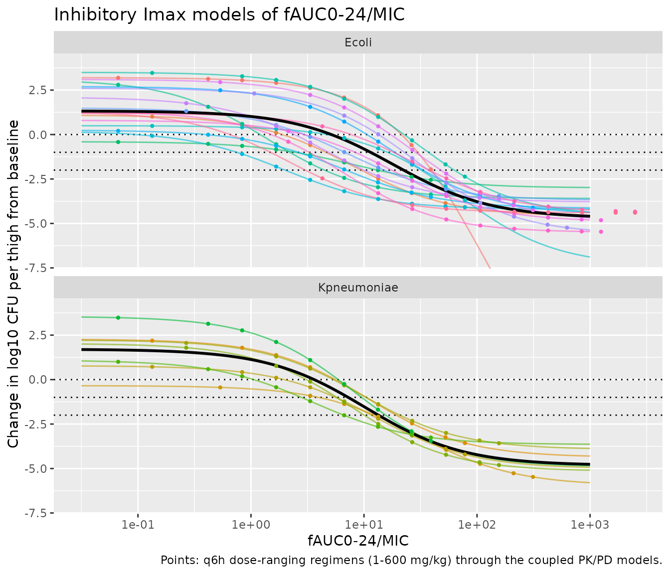
Replicates the fitted lines of Figures S6 and S7 (black) with the per-isolate fits of Figures S8 and S9 (colour).
Using a per-isolate or pooled model directly
mod <- rxode2::rxode(readModelDb("Singley_2026_gepotidacin_Ecoli_ATCC25922"))
ev <- dplyr::bind_rows(lapply(seq_along(pd_doses), function(i) {
  make_events(pd_doses[i], c(0, 24), n_doses = 4, id = i)
}))
rxode2::rxSolve(mod, events = ev, keep = "dose_mgkg") |>
  as.data.frame() |>
  dplyr::filter(time == 24) |>
  dplyr::select(dose_mgkg, fauc_0_24, fauc_mic, dlog10cfu, log_cfu) |>
  dplyr::rename(
    "Dose (mg/kg q6h)" = dose_mgkg, "fAUC0-24 (ug*h/mL)" = fauc_0_24,
    "fAUC0-24/MIC" = fauc_mic, "Change (log10 CFU)" = dlog10cfu,
    "Burden at 24 h (log10 CFU)" = log_cfu
  ) |>
  knitr::kable(digits = 2, caption = "E. coli ATCC 25922 (MIC 1 ug/mL): predicted 24 h response by dose.")
#> Warning: multi-subject simulation without without 'omega'| Dose (mg/kg q6h) | fAUC0-24 (ug*h/mL) | fAUC0-24/MIC | Change (log10 CFU) | Burden at 24 h (log10 CFU) |
|---|---|---|---|---|
| 1.00 | 1.07 | 1.07 | 2.31 | 8.81 |
| 6.25 | 6.68 | 6.68 | 1.06 | 7.56 |
| 12.50 | 13.37 | 13.37 | 0.01 | 6.51 |
| 25.00 | 26.73 | 26.73 | -1.33 | 5.17 |
| 50.00 | 53.45 | 53.45 | -2.72 | 3.78 |
| 100.00 | 106.77 | 106.77 | -3.85 | 2.65 |
| 200.00 | 212.64 | 212.64 | -4.62 | 1.88 |
| 400.00 | 420.91 | 420.91 | -5.07 | 1.43 |
| 600.00 | 624.89 | 624.89 | -5.24 | 1.26 |
For the pooled fits, set mic to the isolate of interest,
e.g. rxode2::ini(mod, mic = fixed(2)); its default is the
species MIC90.
Assumptions and deviations
-
Free concentrations. The paper says total
concentrations were converted to free values with a fixed 24% protein
binding but not whether before fitting or after simulating. The
published parameters predict free concentrations directly: they
reproduce the free-drug Table S2 within 3% without any unbound-fraction
factor (with the factor every row would be 24% low), and the predictions
axis of the NPDE diagnostic (Figure S4) spans the free-drug range of
Figure 1.
Ccis therefore the free concentration and no unbound fraction appears in the models. - Dose unit and body weight. Table S1 gives CL and V in L and L/h, and the Figure S1 equation normalises the dose by 2.7. The dose is therefore in mg per mouse, and 2.7 mg is 100 mg/kg in a 27 g mouse. Doses in mg/kg are converted here with 27 g (the study mice weighed 27-28 g; a 28 g mouse changes exposure by 4%).
-
Untreated controls. The dose term
(DOSE / 2.7)^-0.437is undefined atDOSE = 0. Simulate a vehicle control with no dose records and any positiveDOSE; the index is then 0 and the change equalse0. -
Baseline burden.
log10_cfu0is the nominal 6.5 log10 CFU per thigh the inocula were tailored to; per-isolate baselines are not reported. The fitted endpoint is the change from baseline,dlog10cfu, which does not depend on it. - Typical PK in the PK/PD models. The authors derived the fAUC of each dose group from typical-value simulations (“simulating mean PK profiles”), so the PK/PD models carry no between-subject variability.
-
No PD residual error. Figures S6-S9 report AIC and
R^2 but no residual standard deviation, so
addSdis fixed at 0. -
Default MIC of the pooled fits. The pooled fits
apply to any isolate through fAUC/MIC; their
micdefaults to the species MIC90 in isolates from two global, large-scale uUTI trials (4 ug/mL E. coli, 16 ug/mL K. pneumoniae), which the paper cites when selecting isolates. - Excluded fits. The fAUC (not MIC-normalised), fCmax/MIC, %fT>MIC and four-parameter fits of Table S4 and the right-hand fAUC panels of Figures S6-S9 were index-selection comparisons and are not packaged.
-
Number of animals. The paper reports three mice per
study, dose and time point for PK and five per group for efficacy, but
not the totals, so
n_subjectsis missing.