Cefaclor (Jeong 2021) • nlmixr2lib

Model and source

Citation: Jeong SH, Jang JH, Cho HY, Lee YB. (2021). Population Pharmacokinetic Analysis of Cefaclor in Healthy Korean Subjects. Pharmaceutics 13(5):754. doi:10.3390/pharmaceutics13050754.
Description: Population pharmacokinetic model for cefaclor after a single 250 mg oral capsule (Ceclor) in healthy adult Korean males: one compartment with first-order absorption, an absorption lag time and first-order elimination. Creatinine clearance (Cockcroft-Gault, raw mL/min) enters apparent clearance and body weight enters apparent volume, both as power functions normalized to the cohort medians (110.92 mL/min and 66.05 kg).
Article: https://doi.org/10.3390/pharmaceutics13050754 (open access)

Population

Jeong 2021 pooled the reference-formulation (Ceclor capsule) arms of two randomized, single-dose, open-label, two-way crossover bioequivalence studies of cefaclor in 48 healthy Korean men (Section 2.1). Each subject took a single 250 mg capsule with 240 mL of water and was sampled at 0, 0.25, 0.5, 0.75, 1, 1.25, 1.5, 2, 2.5, 3, 4 and 5 h (Section 2.2), giving 521 plasma concentrations measured by HPLC-UV (LLOQ 0.1 ug/mL; samples below the LLOQ were treated as missing). Table 1 reports age 19-26 years (median 23), body weight 50.0-88.7 kg (median 66.05, mean 67.31 +/- 8.46), serum creatinine 0.70-1.30 mg/dL (mean 0.97 +/- 0.12) and Cockcroft-Gault creatinine clearance 67.50-170.42 mL/min (median 110.92, mean 114.97 +/- 20.86). The model was fit in Phoenix NLME 8.3 by FOCE with extended least squares.

The same information is available programmatically via readModelDb("Jeong_2021_cefaclor")()$population.

Source trace

Every ini() value carries an in-file comment pointing to its source. The table collects them in one place.

Equation / parameter	Value	Source location
Structure: one compartment, first-order absorption with lag time, first-order elimination	–	Section 3.4; Table 3 model 02; Figure 3
`lka` (tvKa)	log(5.203) 1/h	Table 5
`lvc` (tvV/F)	log(22593.260 / 1000) L	Table 5 (printed in mL)
`lcl` (tvCL/F)	log(27166.883 / 1000) L/h	Table 5 (printed in mL/h)
`ltlag` (tvTlag)	log(0.245) h	Table 5
`e_crcl_cl` (dCL/FdCrCl)	0.436	Table 5
`e_wt_vc` (dV/FdWeight)	0.581	Table 5
`etalvc` (omega^2 V/F)	0.011	Table 5
`etalcl` (omega^2 CL/F)	0.034	Table 5
`etalka` (omega^2 Ka)	0.971	Table 5
No IIV on Tlag	–	Table 3 step 02-01-04 ‘Remove IIV Tlag’ (selected)
`propSd` (sigma)	0.270	Table 5; proportional model selected at Table 3 step 02-01
`vc = tvV/F * (WT / 66.05)^e_wt_vc * exp(eta)`	–	Section 3.4 final-model equation
`cl = tvCL/F * (CRCL / 110.92)^e_crcl_cl * exp(eta)`	–	Section 3.4 final-model equation
`ka = tvKa * exp(eta)`; `tlag = tvTlag`	–	Section 3.4 final-model equation
Centring values 66.05 kg and 110.92 mL/min	–	Table 1 medians

mod <- readModelDb("Jeong_2021_cefaclor")
modUi <- rxode2::rxode(mod)
#> ℹ parameter labels from comments will be replaced by 'label()'
# An ODE with a cl/vc pair must stay an ODE, not an auto-solved linCmt().
stopifnot(is.null(modUi$linCmt))

Typical-value checks

These are deterministic: a single typical subject at the Table 1 median covariates with all random effects zeroed. The one-compartment oral model with a lag has a closed form, so the solved profile is checked against it, and the identity CL/F * AUC(0-inf) = Dose is checked with PKNCA.

dose <- 250 # mg
typCov <- data.frame(id = 1L, WT = 66.05, CRCL = 110.92)
tDense <- sort(unique(c(seq(0, 1, by = 0.005), seq(1, 24, by = 0.05))))

evTyp <- rxode2::et(amt = dose, cmt = "depot") |>
  rxode2::et(tDense, cmt = "central") |>
  as.data.frame() |>
  dplyr::mutate(id = 1L)
evTyp <- dplyr::left_join(evTyp, typCov, by = "id")

typSim <- rxode2::rxSolve(
  rxode2::zeroRe(mod),
  events = evTyp, rtol = 1e-10, atol = 1e-12, returnType = "data.frame"
)
#> ℹ parameter labels from comments will be replaced by 'label()'
#> ℹ omega/sigma items treated as zero: 'etalvc', 'etalcl', 'etalka'
# A single-subject solve returns no id column; PKNCA needs one.
typSim$id <- 1L

ka <- 5.203
vc <- 22593.260 / 1000
cl <- 27166.883 / 1000
tlag <- 0.245
kel <- cl / vc
closedForm <- function(t) {
  tt <- pmax(t - tlag, 0)
  dose * ka / (vc * (ka - kel)) * (exp(-kel * tt) - exp(-ka * tt))
}
relErr <- with(
  typSim[typSim$time > tlag + 0.05, ],
  max(abs(Cc / closedForm(time) - 1))
)
relErr
#> [1] 5.69256e-07
stopifnot(relErr < 1e-6)

tmaxTyp <- tlag + log(ka / kel) / (ka - kel)
typTable <- data.frame(
  Quantity = c("CL/F (L/h)", "V/F (L)", "kel (1/h)", "t1/2 (h)", "Tmax (h)", "Cmax (ug/mL)", "AUC0-inf (ug*h/mL)"),
  Value = signif(c(cl, vc, kel, log(2) / kel, tmaxTyp, closedForm(tmaxTyp), dose / cl), 4)
)
knitr::kable(typTable, caption = "Typical-value derived quantities at the median covariates.")

Typical-value derived quantities at the median covariates.
Quantity	Value
CL/F (L/h)	27.1700
V/F (L)	22.5900
kel (1/h)	1.2020
t1/2 (h)	0.5765
Tmax (h)	0.6112
Cmax (ug/mL)	7.1240
AUC0-inf (ug*h/mL)	9.2020


typNca <- PKNCA::pk.nca(PKNCA::PKNCAdata(
  PKNCA::PKNCAconc(
    typSim |> dplyr::filter(!is.na(Cc)) |> dplyr::mutate(treatment = "typical"),
    Cc ~ time | treatment + id
  ),
  PKNCA::PKNCAdose(
    evTyp |> dplyr::filter(evid == 1) |> dplyr::mutate(treatment = "typical"),
    amt ~ time | treatment + id
  ),
  intervals = data.frame(start = 0, end = Inf, aucinf.obs = TRUE)
))
aucTyp <- as.data.frame(typNca$result)$PPORRES[
  as.data.frame(typNca$result)$PPTESTCD == "aucinf.obs"
]
stopifnot(length(aucTyp) == 1L)
# 24 h is > 40 half-lives; the residual is trapezoid error only.
stopifnot(abs(cl * aucTyp / dose - 1) < 1e-3)

The covariate model is checked at the edges of the Table 1 ranges against the power functions of the Section 3.4 equation.

edge <- data.frame(
  id = 1:4,
  WT = c(50.0, 88.7, 66.05, 66.05),
  CRCL = c(110.92, 110.92, 67.50, 170.42)
)
evEdge <- merge(
  data.frame(id = 1:4, time = 0, amt = dose, evid = 1L, cmt = "depot"),
  edge,
  by = "id"
)
evEdge <- rbind(
  evEdge,
  merge(data.frame(id = 1:4, time = 1, amt = 0, evid = 0L, cmt = "central"), edge, by = "id")
)
evEdge <- evEdge[order(evEdge$id, evEdge$time, -evEdge$evid), ]
edgeSim <- rxode2::rxSolve(rxode2::zeroRe(mod), events = evEdge, returnType = "data.frame")
#> ℹ parameter labels from comments will be replaced by 'label()'
#> ℹ omega/sigma items treated as zero: 'etalvc', 'etalcl', 'etalka'
#> Warning: multi-subject simulation without without 'omega'
edgeSim <- edgeSim[edgeSim$time == 1, ]
expectedV <- vc * (edge$WT / 66.05)^0.581
expectedCl <- cl * (edge$CRCL / 110.92)^0.436
stopifnot(
  nrow(edgeSim) == 4L,
  max(abs(edgeSim$vc / expectedV - 1)) < 1e-10,
  max(abs(edgeSim$cl / expectedCl - 1)) < 1e-10
)
knitr::kable(
  data.frame(edge, vc = signif(edgeSim$vc, 4), cl = signif(edgeSim$cl, 4)) |>
    dplyr::rename("V/F (L)" = vc, "CL/F (L/h)" = cl, "CrCl (mL/min)" = CRCL, "Weight (kg)" = WT),
  caption = "Individual V/F and CL/F at the edges of the observed covariate ranges (random effects zeroed)."
)

Individual V/F and CL/F at the edges of the observed covariate ranges (random effects zeroed).
id	Weight (kg)	CrCl (mL/min)	V/F (L)	CL/F (L/h)
1	50.00	110.92	19.22	27.17
2	88.70	110.92	26.81	27.17
3	66.05	67.50	22.59	21.88
4	66.05	170.42	22.59	32.76

Across the observed CrCl range CL/F varies from 80% to 121% of the typical value, and across the observed weight range V/F varies from 85% to 119%.

Virtual cohort

Table 1 gives the marginal distributions but not the joint one. Because CrCl is itself a Cockcroft-Gault function of age, weight and serum creatinine, the cohort draws those three inputs and computes CrCl from them (male form), which reproduces the weight-CrCl correlation that independent draws would miss. Each input is drawn from a normal distribution with the Table 1 mean and SD and redrawn until it falls inside the Table 1 range.

rxode2::rxSetSeed(20210519)
set.seed(20210519)
nSub <- 200L

drawInRange <- function(n, mean, sd, lo, hi) {
  x <- stats::rnorm(n, mean, sd)
  bad <- x < lo | x > hi
  while (any(bad)) {
    x[bad] <- stats::rnorm(sum(bad), mean, sd)
    bad <- x < lo | x > hi
  }
  x
}

cohort <- data.frame(
  id = seq_len(nSub),
  AGE = drawInRange(nSub, 23.00, 1.44, 19, 26),
  WT = drawInRange(nSub, 67.31, 8.46, 50.0, 88.7),
  SCR = drawInRange(nSub, 0.97, 0.12, 0.70, 1.30)
) |>
  dplyr::mutate(CRCL = (140 - AGE) * WT / (72 * SCR))

cohortSummary <- data.frame(
  Covariate = c("Weight (kg)", "CrCl (mL/min)"),
  Paper = c("66.05 (50.00-88.70)", "110.92 (67.50-170.42)"),
  Simulated = c(
    sprintf("%.2f (%.2f-%.2f)", median(cohort$WT), min(cohort$WT), max(cohort$WT)),
    sprintf("%.2f (%.2f-%.2f)", median(cohort$CRCL), min(cohort$CRCL), max(cohort$CRCL))
  )
)
knitr::kable(cohortSummary, caption = "Median (range): Table 1 vs the virtual cohort.")

Median (range): Table 1 vs the virtual cohort.
Covariate	Paper	Simulated
Weight (kg)	66.05 (50.00-88.70)	68.64 (52.66-88.43)
CrCl (mL/min)	110.92 (67.50-170.42)	113.99 (77.17-175.39)

# A Cockcroft-Gault cohort built from the Table 1 inputs should centre near the
# Table 1 CrCl median; a unit slip (e.g. mg/dL vs umol/L) moves it ~88-fold.
stopifnot(abs(median(cohort$CRCL) / 110.92 - 1) < 0.1)

Simulation

paperTimes <- c(0, 0.25, 0.5, 0.75, 1, 1.25, 1.5, 2, 2.5, 3, 4, 5)
obsTimes <- sort(unique(c(paperTimes, seq(0, 6, by = 0.05))))

events <- dplyr::bind_rows(
  data.frame(id = cohort$id, time = 0, amt = dose, evid = 1L, cmt = "depot"),
  tidyr::expand_grid(id = cohort$id, time = obsTimes) |>
    dplyr::mutate(amt = 0, evid = 0L, cmt = "central")
) |>
  dplyr::left_join(cohort |> dplyr::select(id, WT, CRCL), by = "id") |>
  dplyr::mutate(treatment = "250 mg") |>
  dplyr::arrange(id, time, dplyr::desc(evid))

sim <- rxode2::rxSolve(mod, events = events, returnType = "data.frame", keep = "treatment")
#> ℹ parameter labels from comments will be replaced by 'label()'
stopifnot(
  all(is.finite(sim$Cc)),
  all(sim$Cc >= -1e-6 * max(sim$Cc))
)

Figure 1: mean concentration-time profile

Figure 1 of Jeong 2021 shows the observed mean +/- SD plasma cefaclor concentrations on a log scale at the sampling times. The simulated equivalent uses the residual-error-perturbed concentrations (sim) at the same times, with values below the 0.1 ug/mL LLOQ removed as in the paper.

lloq <- 0.1
fig1 <- sim[sim$time %in% paperTimes & sim$time > 0, ] |>
  dplyr::filter(sim >= lloq) |>
  dplyr::group_by(time) |>
  dplyr::summarise(mean = mean(sim), sd = stats::sd(sim), .groups = "drop")
ggplot(fig1, aes(time, mean)) +
  geom_errorbar(aes(ymin = pmax(mean - sd, lloq), ymax = mean + sd), width = 0.08) +
  geom_line() +
  geom_point() +
  scale_y_log10() +
  labs(x = "Time after dose (h)", y = "Cefaclor concentration (ug/mL)")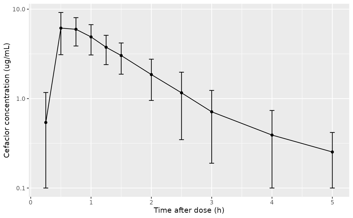

Replicates Figure 1 of Jeong 2021: mean +/- SD cefaclor concentration after a single 250 mg oral dose (simulated, n = 200).

Figure 5: visual predictive check

vpc <- sim |>
  dplyr::group_by(time) |>
  dplyr::summarise(
    p05 = stats::quantile(sim, 0.05),
    p50 = stats::quantile(sim, 0.50),
    p95 = stats::quantile(sim, 0.95),
    .groups = "drop"
  )
ggplot(vpc, aes(time)) +
  geom_ribbon(aes(ymin = p05, ymax = p95), alpha = 0.25) +
  geom_line(aes(y = p50)) +
  geom_line(aes(y = p05), linetype = "dashed") +
  geom_line(aes(y = p95), linetype = "dashed") +
  labs(x = "Time after dose (h)", y = "Cefaclor concentration (ug/mL)")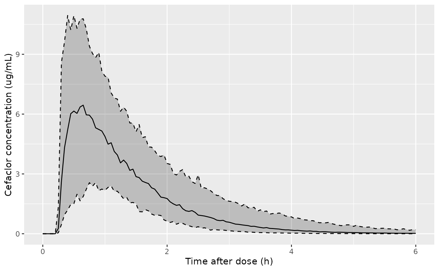

Replicates the prediction intervals of Figure 5 of Jeong 2021: 5th, 50th and 95th percentiles of simulated cefaclor concentrations (with residual error).

PKNCA validation

The NCA is run on the paper’s sampling schedule (0-5 h) using the simulated observations with residual error, and with samples after time zero that fall below the 0.1 ug/mL LLOQ removed, as Section 3.3 describes. This mirrors the design behind Table 2.

simSchedule <- sim[sim$time %in% paperTimes, , drop = FALSE]
simSchedule$Cobs <- ifelse(simSchedule$time == 0, 0, simSchedule$sim)
simSchedule <- simSchedule[simSchedule$time == 0 | simSchedule$Cobs >= lloq, ]

simNca <- simSchedule |>
  dplyr::filter(!is.na(Cobs)) |>
  dplyr::select(id, time, Cobs, treatment)
# Guarantee a time-zero record per subject (pre-dose concentration is zero).
simNca <- dplyr::bind_rows(
  simNca,
  simNca |> dplyr::distinct(id, treatment) |> dplyr::mutate(time = 0, Cobs = 0)
) |>
  dplyr::distinct(id, time, .keep_all = TRUE) |>
  dplyr::arrange(id, time)

doseDf <- events |>
  dplyr::filter(evid == 1L) |>
  dplyr::select(id, time, amt, treatment)

concObj <- PKNCA::PKNCAconc(simNca, Cobs ~ time | treatment + id, concu = "ug/mL", timeu = "h")
doseObj <- PKNCA::PKNCAdose(doseDf, amt ~ time | treatment + id, doseu = "mg")
intervals <- data.frame(
  start = 0, end = Inf,
  cmax = TRUE, tmax = TRUE, auclast = TRUE, aucinf.obs = TRUE, half.life = TRUE
)
ncaRes <- PKNCA::pk.nca(PKNCA::PKNCAdata(concObj, doseObj, intervals = intervals))

Comparison against published NCA

Jeong 2021 Table 2 reports arithmetic means, so the simulated per-subject NCA values are summarised by their mean before comparison.

ncaLong <- as.data.frame(ncaRes$result) |>
  dplyr::filter(
    PPTESTCD %in% c("cmax", "tmax", "auclast", "aucinf.obs", "half.life"),
    is.finite(PPORRES)
  )
simMeans <- ncaLong |>
  dplyr::group_by(treatment, PPTESTCD) |>
  dplyr::summarise(PPORRES = mean(PPORRES), .groups = "drop")
stopifnot(nrow(simMeans) == 5L)

published <- data.frame(
  treatment = "250 mg",
  cmax = 7.87, tmax = 0.80, auclast = 9.64, aucinf.obs = 9.83, half.life = 0.68
)

cmp <- nlmixr2lib::ncaComparisonTable(
  simulated = simMeans,
  reference = published,
  by = "treatment",
  units = c(cmax = "ug/mL", tmax = "h", auclast = "ug*h/mL", aucinf.obs = "ug*h/mL", half.life = "h"),
  tolerance_pct = 20
)
knitr::kable(
  cmp,
  caption = "Mean simulated NCA vs Jeong 2021 Table 2 (mean, n = 48). * marks a difference above 20%.",
  align = c("l", "l", "r", "r", "r")
)

Mean simulated NCA vs Jeong 2021 Table 2 (mean, n = 48). * marks a difference above 20%.
NCA parameter	treatment	Reference	Simulated	% diff
Cmax (ug/mL)	250 mg	7.87	7.48	-5.0%
Tmax (h)	250 mg	0.8	0.752	-5.9%
AUC0-∞ (obs) (ug*h/mL)	250 mg	9.83	8.82	-10.3%
AUClast (ug*h/mL)	250 mg	9.64	8.56	-11.2%
t½ (h)	250 mg	0.68	0.663	-2.5%

pctDiff <- function(code) {
  v <- simMeans$PPORRES[simMeans$PPTESTCD == code]
  if (length(v) != 1L) stop("no unique simulated value for ", code)
  100 * (v / published[[code]] - 1)
}
# AUC is set by Dose / (CL/F): a mis-transcribed clearance, a mL-vs-L slip or a
# wrong dose moves it by tens of percent or orders of magnitude. The expected
# difference is about -10% (-6% from the published typical CL/F, 250 / 27.17 =
# 9.20 vs 9.83 ug*h/mL, and about -4% from the sparse censored NCA design; see
# below). The standard error of a 200-subject mean AUC is about 2%, so 20%
# leaves several standard errors of headroom while still failing on any
# transcription error that moves CL/F by more than about 10%.
stopifnot(
  abs(pctDiff("aucinf.obs")) < 20,
  abs(pctDiff("auclast")) < 20,
  abs(pctDiff("cmax")) < 20
)

To separate the model from the sampling design, the table below compares the NCA estimates with the “true” per-subject values implied by each simulated subject’s parameters (AUC = Dose / CL/F, t1/2 = ln 2 * V/F / CL/F).

ind <- sim |>
  dplyr::group_by(id) |>
  dplyr::summarise(cl = dplyr::first(cl), vc = dplyr::first(vc), .groups = "drop")
trueAuc <- mean(dose / ind$cl)
trueHl <- mean(log(2) * ind$vc / ind$cl)
nca <- function(code) simMeans$PPORRES[simMeans$PPTESTCD == code]
knitr::kable(
  data.frame(
    Quantity = c("AUC0-inf (ug*h/mL)", "t1/2 (h)"),
    Published = c(9.83, 0.68),
    NCA = signif(c(nca("aucinf.obs"), nca("half.life")), 3),
    True = signif(c(trueAuc, trueHl), 3)
  ) |>
    dplyr::rename(
      "Jeong 2021 Table 2" = Published,
      "Simulated NCA (paper design)" = NCA,
      "Simulated, from individual parameters" = True
    ),
  caption = "Mean AUC and half-life: published NCA, NCA of the simulated observations, and the values implied by the simulated individual parameters."
)

Mean AUC and half-life: published NCA, NCA of the simulated observations, and the values implied by the simulated individual parameters.
Quantity	Jeong 2021 Table 2	Simulated NCA (paper design)	Simulated, from individual parameters
AUC0-inf (ug*h/mL)	9.83	8.820	9.20
t1/2 (h)	0.68	0.663	0.59

# Structural: the true mean AUC is Dose / CL/F averaged over the cohort; the
# typical value is 250 / 27.17 = 9.20 ug*h/mL, and the lognormal CL/F IIV
# (omega^2 = 0.034) and the cohort's CrCl spread move the mean by only a few percent.
stopifnot(abs(trueAuc / (dose / cl) - 1) < 0.1)

Cmax and Tmax are reproduced within 6%, and the NCA half-life within 3%. The NCA AUC is about 10% below the published mean. About 4 of those points come from the design: the NCA of the simulated sparse, noisy, LLOQ-censored 0-5 h profiles falls below the AUC implied by the individual clearances. The rest reflects the published fit itself: the popPK typical CL/F (27.17 L/h) gives 250 / 27.17 = 9.20 ug*h/mL, 6% below the published mean AUC of 9.83. The same design effect explains the half-life: the individual parameters imply a mean half-life of about 0.59 h (typical ln 2 * 22.59 / 27.17 = 0.58 h), but a terminal slope fitted to noisy 0-5 h samples reads longer, near the published NCA value of 0.68 h. Tmax depends on where the absorption peak falls on the 0.25 h grid and on the large Ka variability (omega^2 = 0.971), so it is shown but not gated.

Assumptions and deviations

Units. Table 5 prints V/F in mL and CL/F in mL/h. They are divided by 1000 in the model so that a dose in mg gives a concentration in mg/L, which equals the paper’s ug/mL.
Residual-error scale. Table 5 reports the proportional residual error as sigma = 0.270. Phoenix NLME parameterises the residual error by its standard deviation, so the value is used directly as propSd.
IIV values. Table 5 prints omega^2 to three decimals. The IIV (%) column equals 100 * sqrt(omega^2) (for example sqrt(0.971) = 0.985, printed 98.534%), which confirms the column is a variance; the printed variances are used as-is.
CrCl. Cockcroft-Gault creatinine clearance in raw mL/min (not normalised to 1.73 m^2), as in the paper.
Virtual cohort. Only marginal means, SDs and ranges are published. Age, weight and serum creatinine are drawn independently from truncated normal distributions and CrCl is computed from them with the male Cockcroft-Gault equation.
Population scope. The model was fit to healthy young Korean men with CrCl of 67.5-170.4 mL/min. The authors note that its prediction for renal impairment is untested.
Errata. No erratum or correction to Jeong 2021 was found in a EuropePMC search on 2026-09-28.