Model and source
- Citation: Wu YE, Kou C, Li X, Tang BH, Yao BF, Hao GX, Zheng Y, van den Anker J, You DP, Shen AD, Zhao W. Developmental Population Pharmacokinetics-Pharmacodynamics of Meropenem in Chinese Neonates and Young Infants: Dosing Recommendations for Late-Onset Sepsis. Children (Basel). 2022;9(12):1998. doi:10.3390/children9121998
- Description: One-compartment IV-infusion population PK model for meropenem in Chinese neonates and young infants (Wu 2022). V scales linearly with current body weight (reference 2.68 kg); CL scales allometrically with current body weight (fixed exponent 0.75) and with a maturation factor that is a power function of postnatal age (reference 12 days) times a power function of gestational age (reference 36.5 weeks). IIV on V and CL; proportional residual error.
- Article: Children (Basel) 2022;9(12):1998
Population
Wu 2022 pooled 110 opportunistic (scavenged) meropenem plasma
concentrations from 78 Chinese neonates and young infants with bacterial
infection, treated at the Children’s Hospital of Hebei Province and
Beijing Children’s Hospital (Wu 2022 Section 2.1, Section 3.1).
Inclusion required a postmenstrual age (PMA) below 48 weeks. Table 1
reports a median (range) postnatal age (PNA) of 12 days (1-113),
gestational age (GA) of 36.5 weeks (26.3-42.1), PMA of 38.2 weeks
(27.4-46.1), birth weight of 2500 g (480-4100) and current weight (CW)
of 2680 g (980-5310). Doses were 9.3-40.4 mg/kg (median 19.7 mg/kg) per
administration. Forty-three infants had GA <= 37 weeks and 35 had GA
> 37 weeks (Section 2.6). Sex distribution is not reported. The same
information is available programmatically via
rxode2::rxode(readModelDb("Wu_2022_meropenem"))$population.
Source trace
| Equation / parameter | Value | Source location |
|---|---|---|
| One-compartment, first-order elimination | n/a | Section 3.2 paragraph 1 |
lvc (theta1) |
1.63 L | Table 2, row ‘theta1’ under V |
lcl (theta2) |
0.503 L/h | Table 2, row ‘theta2’ under CL |
e_wt_vc |
1 (fixed) | Section 3.2 paragraph 2 (‘allometric coefficients of 1 for V’); Table 2 V equation |
e_wt_cl |
0.75 (fixed) | Section 3.2 paragraph 2; Table 2 CL equation |
e_pna_cl (theta3) |
0.209 | Table 2, row ‘theta3’ (F_age) |
e_ga_cl (theta4) |
2.14 | Table 2, row ‘theta4’ (F_age) |
etalvc |
0.03017 = log(0.175^2 + 1) | Table 2, IIV V 17.5% |
etalcl |
0.22957 = log(0.508^2 + 1) | Table 2, IIV CL 50.8% |
propSd |
0.288 | Table 2, residual variability 28.8%; Section 3.2 (proportional) |
| V = theta1 * (CW/2680) | n/a | Table 2 |
| CL = theta2 * (CW/2680)^0.75 * F_age | n/a | Table 2 |
| F_age = (PNA/12)^theta3 * (GA/36.5)^theta4 | n/a | Table 2 |
| Reference values 2680 g, 36.5 weeks, 12 days | n/a | Table 2 footnote (cohort medians) |
| Free fraction 0.98, target 70% fT > MIC, MIC 8 mg/L | n/a | Section 2.6 |
Virtual cohort
The individual covariates are not published, so the cohort is generated from the Table 1 summaries, one cohort per GA subgroup used in the paper’s dosing simulations (GA <= 37 weeks and GA > 37 weeks). GA is drawn from a normal distribution centred on the median (36.5 weeks, SD 4.65 weeks) truncated to the subgroup’s share of the 26.3-42.1 week range; PNA from a log-normal with the Table 1 median (12 days) and a log-scale SD chosen to reproduce the Table 1 mean (17.6 days), truncated to 1-113 days. Current weight is linked to PMA by a linear relation built from the Table 1 means and SDs of CW and PMA with an assumed correlation of 0.85, truncated to the observed 980-5310 g range.
set.seed(20221219)

n_per_group <- 200L

rtrunc_norm <- function(n, mean, sd, lower, upper) {
  out <- numeric(0)
  while (length(out) < n) {
    x <- rnorm(4L * n, mean, sd)
    out <- c(out, x[x >= lower & x <= upper])
  }
  out[seq_len(n)]
}

# PNA: log-normal with median 12 days; mean = median * exp(s^2 / 2) = 17.6
pna_sdlog <- sqrt(2 * log(17.6 / 12))

make_group <- function(group, ga_lower, ga_upper) {
  ga <- rtrunc_norm(n_per_group, 36.5, 4.65, ga_lower, ga_upper)
  pna_d <- rtrunc_norm(n_per_group, log(12), pna_sdlog, log(1), log(113)) |> exp()
  pma <- ga + pna_d / 7
  r <- 0.85
  cw_g <- 2661 + r * 927 / 4.40 * (pma - 37.5) +
    rnorm(n_per_group, 0, 927 * sqrt(1 - r^2))
  cw_g <- pmin(pmax(cw_g, 980), 5310)
  tibble(
    subj = seq_len(n_per_group),
    group = group,
    GA = ga,
    PNA = pna_d / 30.4375, # canonical PNA is in months
    PNA_days = pna_d,
    WT = cw_g / 1000
  )
}

cohort <- bind_rows(
  make_group("GA <= 37 weeks", 26.3, 37),
  make_group("GA > 37 weeks", 37.0001, 42.1)
)

cohort |>
  group_by(group) |>
  summarise(
    N = n(),
    `GA median (weeks)` = median(GA),
    `PNA median (days)` = median(PNA_days),
    `CW median (kg)` = median(WT),
    .groups = "drop"
  ) |>
knitr::kable(digits = 2, caption = "Virtual cohort covariates by GA subgroup.")| group | N | GA median (weeks) | PNA median (days) | CW median (kg) |
|---|---|---|---|---|
| GA <= 37 weeks | 200 | 33.71 | 12.74 | 2.31 |
| GA > 37 weeks | 200 | 39.43 | 10.57 | 3.29 |
Typical-value check against the reported weight-normalised parameters
Section 3.2 reports median (range) individual weight-normalised V of 0.60 (0.51-0.69) L/kg and CL of 0.16 (0.04-0.51) L/h/kg. At the reference subject (CW 2.68 kg, PNA 12 days, GA 36.5 weeks) the model returns exactly theta1 and theta2.
mod <- readModelDb("Wu_2022_meropenem")

ref_ev <- data.frame(
  id = 1L, time = c(0, 1), evid = c(1L, 0L), amt = c(100, 0),
  cmt = "central", WT = 2.68, GA = 36.5, PNA = 12 / 30.4375
)
ref <- rxode2::rxSolve(rxode2::zeroRe(mod), ref_ev) |> as.data.frame()
#> ℹ parameter labels from comments will be replaced by 'label()'
#> ℹ omega/sigma items treated as zero: 'etalvc', 'etalcl'
stopifnot(
  abs(ref$vc[1] / 1.63 - 1) < 1e-6,
  abs(ref$cl[1] / 0.503 - 1) < 1e-6
)
c(V_per_kg = ref$vc[1] / 2.68, CL_per_kg = ref$cl[1] / 2.68)
#>  V_per_kg CL_per_kg
#> 0.6082090 0.1876866
The typical-subject V/kg (0.61 L/kg) matches the reported median of 0.60 L/kg. The typical-subject CL/kg (0.19 L/h/kg) sits above the reported median individual estimate of 0.16 L/h/kg; with 50.8% IIV on CL and the skew of the PNA distribution towards the first two weeks of life the median individual estimate is expected to lie below the reference value.
Simulation
Meropenem is linear in this model, so concentrations scale with dose. The dosing grid of Figure 4 (20-60 mg/kg; twice or three times daily; 1-5 h infusions) is therefore simulated once per frequency and infusion duration at 1 mg/kg and rescaled for each dose level. Six doses are given, and the PTA is evaluated over the sixth dosing interval.
regimens <- expand_grid(tau = c(12, 8), tinf = 1:5) |>
  mutate(reg = row_number())

n_dose <- 6L
dt <- 0.05

build_events <- function(cohort, regimens) {
  design <- cross_join(cohort, regimens) |>
    mutate(id = row_number())
  doses <- design |>
    cross_join(tibble(dose_n = seq_len(n_dose))) |>
    mutate(
      time = (dose_n - 1) * tau,
      evid = 1L,
      amt = 1 * WT, # 1 mg/kg
      rate = amt / tinf,
      cmt = "central"
    )
  obs <- design |>
    cross_join(tibble(k = 0:round(max(regimens$tau) / dt))) |>
    filter(k * dt <= tau + 1e-9) |>
    mutate(
      time = (n_dose - 1) * tau + k * dt,
      evid = 0L, amt = 0, rate = 0, cmt = "central"
    )
  bind_rows(doses, obs) |>
    select(id, time, evid, amt, rate, cmt, WT, GA, PNA, group, tau, tinf, reg) |>
    arrange(id, time, desc(evid))
}

events <- build_events(cohort, regimens)

rxode2::rxSetSeed(20221219)
sim <- rxode2::rxSolve(
  mod,
  events = events,
  keep = c("group", "tau", "tinf", "reg")
) |>
  as.data.frame()
#> ℹ parameter labels from comments will be replaced by 'label()'
stopifnot(!anyNA(sim$Cc))
Replicate Figure 4: probability of target attainment
Target attainment is free concentration (98% of total, Section 2.6) above an MIC of 8 mg/L for at least 70% of the dosing interval.
fu <- 0.98
mic <- 8
dose_levels <- c(20, 30, 40, 50, 60)

# Fraction of the final interval each subject spends above the MIC, per
# dose level (the unit-dose profile scaled by the dose in mg/kg).
ft <- sim |>
  select(id, time, Cc, group, tau, tinf) |>
  cross_join(tibble(dose = dose_levels)) |>
  group_by(id, group, tau, tinf, dose) |>
  summarise(ft_mic = mean(fu * Cc * dose > mic), .groups = "drop")

pta <- ft |>
  group_by(group, tau, tinf, dose) |>
  summarise(PTA = 100 * mean(ft_mic >= 0.7), .groups = "drop") |>
  mutate(freq = ifelse(tau == 12, "BID (q12h)", "TID (q8h)"))
ggplot(pta, aes(tinf, PTA, colour = factor(dose))) +
  geom_line() +
  geom_point() +
  geom_hline(yintercept = 70, linetype = "dashed") +
  facet_grid(freq ~ group) +
  labs(
    x = "Infusion duration (h)",
    y = "PTA, 70% fT > MIC of 8 mg/L (%)",
    colour = "Dose (mg/kg)",
    caption = "Replicates Figure 4 of Wu 2022 with a virtual cohort."
  )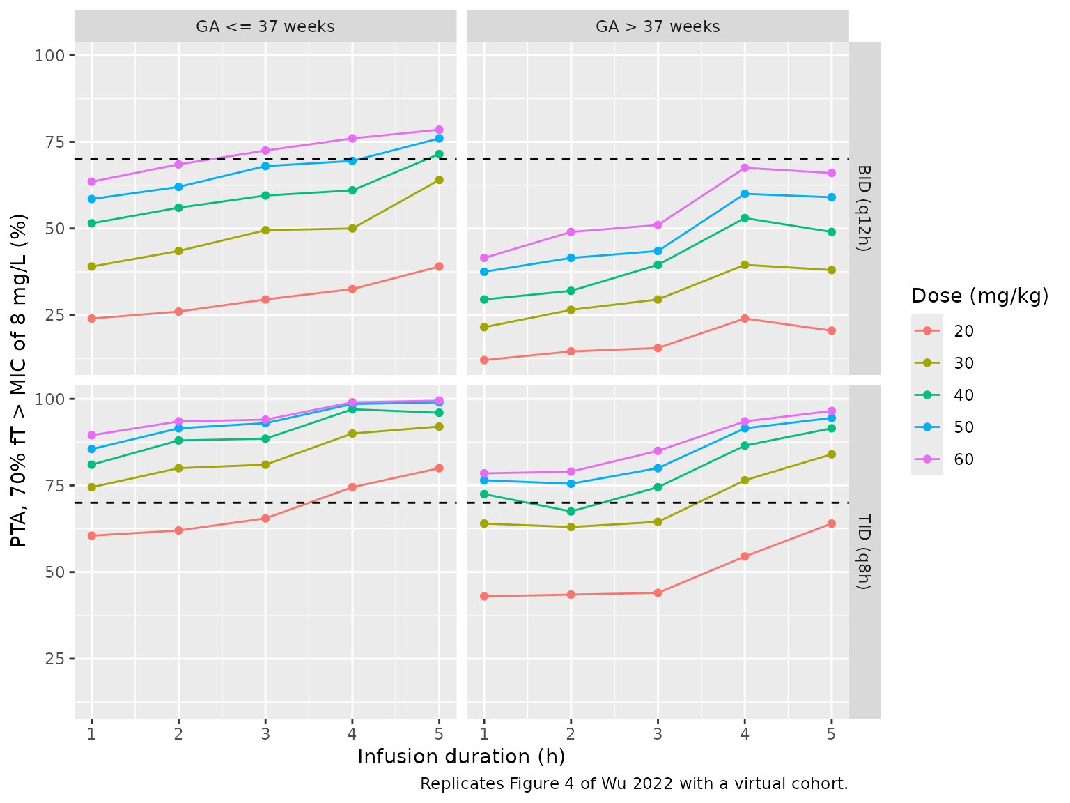
Section 3.4 quotes the PTA of the regimens it recommends. The table compares them with the virtual-cohort values.
published <- tribble(
  ~group,           ~tau, ~tinf, ~dose, ~PTA_published,
  "GA <= 37 weeks",   12,     3,    60,          72.49,
  "GA <= 37 weeks",   12,     4,    50,          73.54,
  "GA <= 37 weeks",   12,     5,    40,          74.09,
  "GA <= 37 weeks",    8,     1,    30,          71.71,
  "GA > 37 weeks",     8,     2,    50,          72.50,
  "GA > 37 weeks",     8,     3,    40,          75.08
)

pta_cmp <- published |>
  inner_join(pta, by = c("group", "tau", "tinf", "dose")) |>
  mutate(diff = PTA - PTA_published)
stopifnot(nrow(pta_cmp) == nrow(published))

pta_cmp |>
  mutate(Regimen = sprintf("%g mg/kg q%gh, %g-h infusion", dose, tau, tinf)) |>
  select(group, Regimen, PTA_published, PTA, diff) |>
  rename(
    "GA subgroup" = group,
    "PTA, Wu 2022 (%)" = PTA_published,
    "PTA, simulated (%)" = PTA,
    "Difference (points)" = diff
  ) |>
knitr::kable(digits = 1, caption = "PTA of the Section 3.4 regimens: published versus virtual cohort.")| GA subgroup | Regimen | PTA, Wu 2022 (%) | PTA, simulated (%) | Difference (points) |
|---|---|---|---|---|
| GA <= 37 weeks | 60 mg/kg q12h, 3-h infusion | 72.5 | 72.5 | 0.0 |
| GA <= 37 weeks | 50 mg/kg q12h, 4-h infusion | 73.5 | 69.5 | -4.0 |
| GA <= 37 weeks | 40 mg/kg q12h, 5-h infusion | 74.1 | 71.5 | -2.6 |
| GA <= 37 weeks | 30 mg/kg q8h, 1-h infusion | 71.7 | 74.5 | 2.8 |
| GA > 37 weeks | 50 mg/kg q8h, 2-h infusion | 72.5 | 75.5 | 3.0 |
| GA > 37 weeks | 40 mg/kg q8h, 3-h infusion | 75.1 | 74.5 | -0.6 |
# The published PTAs come from the authors' own 78 covariate sets; the
# virtual cohort only approximates their joint distribution, and each
# simulated PTA carries a binomial SE of about 3 points at n = 200, so
# the gate is on the centre of the six differences, not their extreme.
# Across four seeds the median difference ranged 0.0 to 3.0 points and the
# median absolute difference 3.1 to 4.3 points. A mis-transcribed CL, V or
# exponent moves these PTAs by tens of points.
stopifnot(
  abs(median(pta_cmp$diff)) < 6,
  median(abs(pta_cmp$diff)) < 8
)
The virtual-cohort PTAs for the six regimens Section 3.4 recommends fall within a few percentage points of the published values, about the size of the binomial Monte Carlo error at 200 subjects per subgroup.
PKNCA validation
Steady-state NCA over the sixth dosing interval for the two regimens the paper recommends (30 mg/kg q8h as a 1-h infusion for GA <= 37 weeks, 40 mg/kg q8h as a 3-h infusion for GA > 37 weeks), solved at the actual doses.
rec <- tribble(
  ~group,           ~dose, ~tau, ~tinf, ~treatment,
  "GA <= 37 weeks",    30,    8,     1, "30 mg/kg q8h 1-h (GA <= 37)",
  "GA > 37 weeks",     40,    8,     3, "40 mg/kg q8h 3-h (GA > 37)"
)

design_rec <- cohort |>
  inner_join(rec, by = "group") |>
  mutate(id = row_number())

dose_rec <- design_rec |>
  cross_join(tibble(dose_n = seq_len(n_dose))) |>
  mutate(
    time = (dose_n - 1) * tau, evid = 1L, amt = dose * WT,
    rate = amt / tinf, cmt = "central"
  )
obs_rec <- design_rec |>
  cross_join(tibble(time = seq(0, n_dose * 8, by = 0.1))) |>
  mutate(evid = 0L, amt = 0, rate = 0, cmt = "central")
events_rec <- bind_rows(dose_rec, obs_rec) |>
  select(id, time, evid, amt, rate, cmt, WT, GA, PNA, treatment, tau) |>
  arrange(id, time, desc(evid))

sim_rec <- rxode2::rxSolve(mod, events = events_rec, keep = c("treatment", "tau")) |>
  as.data.frame()
stopifnot(!anyNA(sim_rec$Cc))
t_start <- (n_dose - 1) * 8
t_end <- n_dose * 8

conc_df <- sim_rec |>
  filter(!is.na(Cc), time >= t_start, time <= t_end) |>
  mutate(Cc = pmax(Cc, 0)) |>
  select(id, time, Cc, treatment)

dose_df <- events_rec |>
  filter(evid == 1, time == t_start) |>
  select(id, time, amt, rate, treatment) |>
  mutate(duration = amt / rate)

conc_obj <- PKNCA::PKNCAconc(conc_df, Cc ~ time | treatment + id,
                             concu = "mg/L", timeu = "h")
dose_obj <- PKNCA::PKNCAdose(dose_df, amt ~ time | treatment + id,
                             doseu = "mg", duration = "duration")
intervals <- data.frame(
  start = t_start, end = t_end,
  cmax = TRUE, tmax = TRUE, cmin = TRUE, auclast = TRUE, cav = TRUE
)
nca_res <- PKNCA::pk.nca(PKNCA::PKNCAdata(conc_obj, dose_obj, intervals = intervals))
knitr::kable(summary(nca_res),
caption = "Simulated steady-state NCA (sixth dosing interval) for the two recommended regimens.")| Interval Start | Interval End | treatment | N | AUClast (h*mg/L) | Cmax (mg/L) | Cmin (mg/L) | Tmax (h) | Cav (mg/L) |
|---|---|---|---|---|---|---|---|---|
| 40 | 48 | 30 mg/kg q8h 1-h (GA <= 37) | 200 | 188 [55.2] | 50.9 [26.6] | 6.31 [218] | 1.00 [1.00, 1.00] | 23.5 [55.2] |
| 40 | 48 | 40 mg/kg q8h 3-h (GA > 37) | 200 | 186 [48.1] | 43.1 [30.6] | 5.83 [196] | 3.00 [3.00, 3.00] | 23.3 [48.1] |
At steady state, AUC over one dosing interval equals dose / CL for each subject. The check below compares PKNCA’s AUC with that identity using each subject’s simulated clearance.
cl_df <- sim_rec |>
  group_by(id) |>
  summarise(cl = first(cl), .groups = "drop")

auc_chk <- as.data.frame(nca_res$result) |>
  filter(PPTESTCD == "auclast") |>
  select(id, treatment, auclast = PPORRES) |>
  inner_join(cl_df, by = "id") |>
  inner_join(dose_df |> select(id, amt), by = "id") |>
  mutate(pct_diff = 100 * (auclast / (amt / cl) - 1))

auc_chk |>
  group_by(treatment) |>
  summarise(
    `Median % difference` = median(pct_diff),
    `90th percentile of abs % difference` = quantile(abs(pct_diff), 0.9),
    .groups = "drop"
  ) |>
knitr::kable(digits = 2, caption = "PKNCA AUC0-tau versus dose / CL.")| treatment | Median % difference | 90th percentile of abs % difference |
|---|---|---|
| 30 mg/kg q8h 1-h (GA <= 37) | -0.01 | 0.15 |
| 40 mg/kg q8h 3-h (GA > 37) | -0.01 | 0.03 |
# After six doses only subjects with the slowest CL are short of steady
# state, and the 0.1-h trapezoid grid adds a small bias. Realised median
# about -0.01% and 90th percentile below 0.2%; a dose, unit or CL error
# shifts every subject by far more than these bounds.
stopifnot(
  abs(median(auc_chk$pct_diff)) < 0.5,
  quantile(abs(auc_chk$pct_diff), 0.9) < 2
)
The paper reports no NCA parameters, so no published-versus-simulated NCA table is shown.
Assumptions and deviations
-
PNA units. The Table 2 footnote describes PNA as
‘postnatal age in weeks’ but, in the same footnote, gives 12 days as the
median PNA used for centring, and Table 1 reports PNA in days (median
12.0). The model therefore takes PNA in days inside the F_age term. The
package’s canonical
PNAcolumn is in months;model()converts with PNA * 30.4375. -
Weight units. The paper uses current weight in
grams centred on 2680 g. The packaged model takes
WTin kg centred on 2.68 kg, which is numerically identical. - IIV conversion. Table 2 reports IIV as a percentage for an exponential model; it is converted with omega^2 = log(CV^2 + 1). Residual variability (28.8%) is encoded as a proportional SD of 0.288.
- Virtual cohort. The paper’s dosing simulations reuse its own 78 covariate sets, which are not published. The virtual cohort here is generated from the Table 1 summaries with an assumed CW-PMA correlation of 0.85, and GA drawn from a normal distribution centred on the median (the published GA distribution is left-skewed, mean 35.0 versus median 36.5 weeks). The simulated PTAs are therefore an approximation of Figure 4, not a replication of the authors’ cohort.
- PTA evaluation window. Section 2.6 does not state which dosing interval the PTA was evaluated on. The sixth interval (steady state for nearly every subject) is used here, without residual error.
- External validation not reproduced. The 16-infant external validation dataset is not published.