Quetiapine cortical dopamine in schizophrenia phenotyped rats (Dias 2024)
Source:vignettes/articles/Dias_2024_quetiapine_rat.Rmd
Dias_2024_quetiapine_rat.Rmd
mod <- rxode2::rxode2(readModelDb("Dias_2024_quetiapine_rat"))
#> ℹ parameter labels from comments will be replaced by 'label()'
Model and source
- Citation: Dias BB, Carreno F, Helfer VE, Olivo LB, Staudt KJ, Paese K, Barreto F, Meyer FS, Herrmann AP, Guterres SS, Rates SMK, de Araujo BV, Troconiz IF, Dalla Costa T. Pharmacokinetic/pharmacodynamic modeling of cortical dopamine concentrations after quetiapine lipid core nanocapsules administration to schizophrenia phenotyped rats. CPT Pharmacometrics Syst Pharmacol. 2024;13(4):638-648. doi:10.1002/psp4.13107. Upstream PK driver (not implemented here): Carreno F et al. J Pharmacol Exp Ther. 2020;375(1):49-58, doi:10.1124/jpet.120.000109.
- Article: https://doi.org/10.1002/psp4.13107 (PMC11015084, open access)
- Supplementary Material S1 supplies Table S1 (the full population parameter set with %RSE, IIV, shrinkage and non-parametric bootstrap CIs) and the complete NM-TRAN control stream for the final model. Both are used as primary sources here.
This is a pharmacodynamic-only model. It has no PK
layer and takes no dosing events: the unbound quetiapine concentration
in medial prefrontal cortex (mPFC) interstitial fluid enters as the
time-varying covariate CU_QTP_BRAIN, exactly as the
authors’ NM-TRAN reads it from the CBRAIN data item. The
driver profiles were generated by the companion semimechanistic popPK
model of Carreno et al. 2020 (doi:10.1124/jpet.120.000109)
and are plotted in this paper’s Figure 4a and Figure S2.
Population
| Field | Value |
|---|---|
| Species | rat (Wistar; naive and prenatal poly(i:c) schizophrenia phenotyped) |
| Subjects | 49 |
| Observations | 924 |
| Female | 49% |
| Disease state | Naive rats and schizophrenia phenotyped rats (SPR). SPR offspring were generated by a single 4 mg/kg i.v. poly(i:c) bolus to pregnant dams at gestational day 15 (naive dams received 2 mL/kg saline); the phenotype was confirmed in adult offspring (PND75) by the prepulse inhibition of the acoustic startle response test. |
| Dose | Single 5 mg/kg intravenous bolus of quetiapine via the lateral caudal vein, given either as a solution (FQ, 5 mg/mL) or as quetiapine lipid core nanocapsules (QLNC, 1 mg/mL). |
| Region | Brazil (Federal University of Rio Grande do Sul, Porto Alegre) |
Dopamine in mPFC extracellular fluid was sampled by intracerebral microdialysis: after a 1 h equilibration, four 20-min baseline dialysates were collected, the animal then received a single 5 mg/kg intravenous bolus, and 15 further 20-min dialysates were collected to 280 min. The four baseline dialysates place the dose at about 1.33 h on the microdialysis clock, which is where the driver profiles in Figure 4a step up.
Source trace
Equations
| Model element | Source location | Form as implemented |
|---|---|---|
| Precursor pool | Eq (1); NM-TRAN DADT(1)
|
d/dt(precursor1) <- kpin - kpout * deff * precursor1 |
| Extracellular dopamine | Eq (2); NM-TRAN DADT(2)
|
d/dt(dopamine) <- kpout * deff * precursor1 - kout * dopamine * modulator |
| Dialysate integral | NM-TRAN DADT(3),
$ERROR AA4 = A(3)/TIN
|
d/dt(auc_dopamine) <- dopamine |
| Negative feedback | Eq (4); NM-TRAN DADT(4)
|
d/dt(modulator) <- kmod * (dopamine / rbase_dopamine - modulator) |
| Effect compartment | NM-TRAN DADT(5) (not printed Eq (3);
see Errata) |
d/dt(effect) <- ke0 * CU_QTP_BRAIN - effect |
| Nanoparticle decay | Eq (5); NM-TRAN DADT(6)
|
d/dt(nano) <- -knp * nano |
| Drug effect | Results text; NM-TRAN DEFF
|
deff <- 1 + eqtp * effect / (1 + nano) |
| Derived release / reuptake | Results text; NM-TRAN KBASE, KEL
|
kpout <- kpin / rbase_precursor1;
kout <- kpin / rbase_dopamine
|
| PPI on EQTP | Eq (6); NM-TRAN TVSLPE
|
eqtp <- exp(leqtp + eta) * (1 + e_score_ppi_eqtp * (SCORE_PPI - 33.4)) |
| PPI on DA0 | Eq (7); NM-TRAN TVBASE; restated in Discussion |
rbase_dopamine <- exp(lrbase_dopamine + eta) * (1 + e_score_ppi_rbase_dopamine * (SCORE_PPI - 33.4)) |
Parameters
Every value below is a final population estimate from Supplementary
Material S1 Table S1, cross-checked against the NM-TRAN $PK
theta assignments.
| Parameter | File value | Table S1 (%RSE) | Bootstrap median (95% CI) | IIV % | Shrinkage % |
|---|---|---|---|---|---|
| Pool0 (ng/mL) | 1.16 | 1.16 (29) | 1.16 (0.82-1.47) | - | - |
| Kin (ng/mL/h) | 0.313 | 0.313 (22) | 0.311 (0.225-0.428) | 36 | 29 |
| DA0 (ng/mL) | 0.288 | 0.288 (3) | 0.288 (0.274-0.304) | 16 | 8 |
| EQTP (mL/ng) | 37.7 | 37.7 (66) | 39.3 (33.4-59.4) | 51 | 43 |
| Keo (1/h) | 0.418 | 0.418 (50) | 0.436 (0.371-0.661) | 54 | 38 |
| Kmod (1/h) | 0.564 | 0.564 (44) | 0.566 (0.352-0.967) | 62 | 58 |
| KNP (1/h) | 3.34 | 3.34 (17) | 3.22 (2.54-4.32) | - | - |
| NP0 (ng/mL) | 4.7e4 | 4.7e4 (144) | 5.0e4 (6.4e3-8.2e5) | 151 | 38 |
| theta DA0,SPR | 0.0095 | 0.0095 (20) | 0.0093 (0.0056-0.0123) | - | - |
| theta EQTP,SPR | 0.0243 | 0.0243 (47) | 0.0265 (0.0077-0.0407) | - | - |
| Additive SD (ng/mL) | 0.0759 | 0.0759 (5) | 0.0759 (0.0690-0.0821) | - | 7 |
The Table S1 footnote defines the IIV column as “expressed as CV (%)
calculated as omega2 x 100, where omega2 is the standard deviation of
the variance of the random effect”, i.e. the tabulated percentage is 100
times the log-scale SD. The file therefore encodes variances as
(CV% / 100)^2.
Dimensional analysis
| ODE term | Units multiplied out | Required |
|---|---|---|
kpin |
ng/mL/h | ng/mL/h |
kpout * deff * precursor1 |
(1/h)(1)(ng/mL) = ng/mL/h | ng/mL/h |
kout * dopamine * modulator |
(1/h)(ng/mL)(1) = ng/mL/h | ng/mL/h |
dopamine (into auc_dopamine) |
ng/mL | (ng/mL h)/h = ng/mL |
kmod * (dopamine/rbase_dopamine - modulator) |
(1/h)(1) = 1/h | 1/h |
ke0 * CU_QTP_BRAIN |
(1/h)(ng/mL) = ng/mL/h | ng/mL/h |
- effect |
ng/mL, carrying an implicit 1/h | ng/mL/h |
knp * nano |
(1/h)(ng/mL) = ng/mL/h | ng/mL/h |
eqtp * effect |
(mL/ng)(ng/mL) = 1 | 1 (deff is unitless) |
Two consequences are worth stating explicitly. First,
EQTP is dimensionally a reciprocal concentration (mL/ng);
the paper tabulates it without units. Second, the bare
- A(5) in the control stream’s DADT(5) carries
an implicit first-order rate constant of exactly 1 /h; this is what
makes Keo a gain rather than only a delay, and it is why
the effect-compartment form differs from printed Eq (3) (see
Errata).
The externally supplied driver
The paper contains no PK layer, so the unbound brain quetiapine profiles must be supplied. They are published only as figures (Figure 4a, Figure S2), so the values below were digitised from Figure 4a of the rendered article at 400 dpi. They are approximate (roughly +/- 0.01 ng/mL) and are used here only to drive the figure replication; no model parameter is derived from them.
driver <- tibble::tribble(
  ~group,        ~time, ~CU_QTP_BRAIN,
  "FQ-naive",     0.00, 0.000,
  "FQ-naive",     1.33, 0.000,
  "FQ-naive",     1.67, 0.346,
  "FQ-naive",     2.20, 0.335,
  "FQ-naive",     2.80, 0.294,
  "FQ-naive",     3.50, 0.251,
  "FQ-naive",     4.20, 0.209,
  "FQ-naive",     4.90, 0.168,
  "FQ-naive",     5.60, 0.128,
  "FQ-naive",     6.30, 0.105,
  "FQ-SPR",       0.00, 0.000,
  "FQ-SPR",       1.30, 0.000,
  "FQ-SPR",       1.80, 0.197,
  "FQ-SPR",       2.40, 0.191,
  "FQ-SPR",       3.40, 0.168,
  "FQ-SPR",       4.45, 0.140,
  "FQ-SPR",       5.45, 0.114,
  "FQ-SPR",       6.30, 0.094,
  "QLNC-naive",   0.00, 0.000,
  "QLNC-naive",   1.30, 0.000,
  "QLNC-naive",   2.14, 0.341,
  "QLNC-naive",   2.80, 0.284,
  "QLNC-naive",   3.25, 0.272,
  "QLNC-naive",   4.10, 0.248,
  "QLNC-naive",   4.95, 0.225,
  "QLNC-naive",   5.80, 0.201,
  "QLNC-naive",   6.30, 0.195,
  "QLNC-SPR",     0.00, 0.000,
  "QLNC-SPR",     1.30, 0.000,
  "QLNC-SPR",     2.11, 0.311,
  "QLNC-SPR",     2.95, 0.308,
  "QLNC-SPR",     3.80, 0.294,
  "QLNC-SPR",     4.15, 0.289,
  "QLNC-SPR",     4.50, 0.268,
  "QLNC-SPR",     5.30, 0.225,
  "QLNC-SPR",     6.15, 0.189,
  "QLNC-SPR",     6.30, 0.186
)

# Group-level (two-stage) parameter estimates, Table 1. These are the medians
# of the individual estimates within each experimental group and already
# include the PPI covariate effect, so SCORE_PPI is held at PPImd = 33.4
# whenever these are used (making both covariate factors exactly 1).
groupPars <- tibble::tribble(
  ~group,        ~Pool0, ~Kin,   ~DA0,   ~EQTP,  ~Keo,   ~Kmod,  ~KNP,  ~NP0,   ~qlnc,
  "FQ-naive",     2.19,  0.299,  0.298,  37.3,   0.450,  0.529,  3.34,  0,      0,
  "FQ-SPR",       2.07,  0.853,  0.222,  33.6,   0.500,  0.910,  3.34,  0,      0,
  "QLNC-naive",   2.57,  0.609,  0.340,  50.8,   0.568,  0.772,  3.79,  8.4e4,  1,
  "QLNC-SPR",     3.19,  0.913,  0.294,  100.7,  1.01,   1.27,   2.56,  6.3e4,  1
)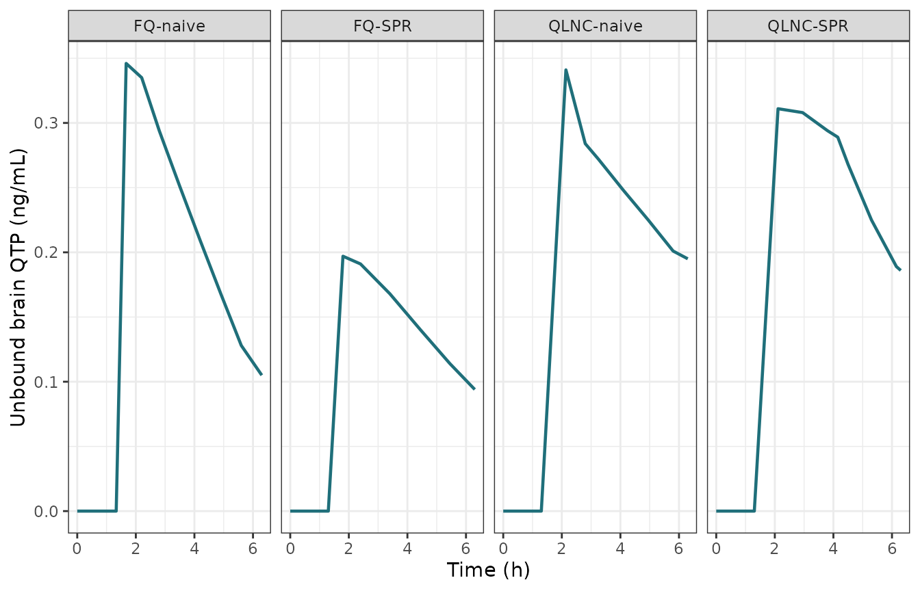
Digitised unbound brain quetiapine driver profiles (replicates the solid Cu,brain curves of Figure 4a of Dias 2024).
# Solve the library model for one experimental group at its Table 1 estimates.
# Covariate effects are neutralised by holding SCORE_PPI at PPImd, so DA0 and
# EQTP enter exactly as tabulated.
solveGroup <- function(g, times = seq(0, 6.3, by = 0.02), inits = NULL) {
  gp <- groupPars[groupPars$group == g, ]
  dv <- driver[driver$group == g, ]
  ev <- data.frame(
    id = 1L,
    time = times,
    amt = NA_real_,
    evid = 0L,
    cmt = "dopamine",
    SCORE_PPI = 33.4,
    FORM_QTP_QLNC = gp$qlnc,
    CU_QTP_BRAIN = stats::approx(dv$time, dv$CU_QTP_BRAIN, xout = times,
                                 rule = 2)$y
  )
  pars <- c(
    lrbase_precursor1 = log(gp$Pool0),
    lkpin = log(gp$Kin),
    lrbase_dopamine = log(gp$DA0),
    leqtp = log(gp$EQTP),
    lke0 = log(gp$Keo),
    lkmod = log(gp$Kmod),
    lknp = log(gp$KNP),
    lnp0 = log(max(gp$NP0, 1)),
    e_score_ppi_rbase_dopamine = 0.0095,
    e_score_ppi_eqtp = 0.0243
  )
  out <- rxode2::rxSolve(mod, ev, params = pars, omega = NA,
                         inits = inits, returnType = "data.frame")
  out$group <- g
  out
}

groups <- groupPars$group
sims <- dplyr::bind_rows(lapply(groups, solveGroup))
Validation
This is an endogenous turnover model, so the validation follows the steady-state / perturbation-recovery / flux-balance pattern rather than NCA. There is no dose and no concentration-time profile of the modelled species to integrate, so PKNCA is not applicable.
1. Drug-free steady state
With no drug the system must sit exactly at the reported baselines
forever: deff is 1, modulator is 1, and both
turnover equations cancel by construction because
kpout = Kin/Pool0 and kout = Kin/DA0.
ssEv <- data.frame(
  id = 1L, time = seq(0, 72, by = 0.5), amt = NA_real_, evid = 0L,
  cmt = "dopamine", SCORE_PPI = 33.4, FORM_QTP_QLNC = 0, CU_QTP_BRAIN = 0
)
ss <- rxode2::rxSolve(mod, ssEv, omega = NA, returnType = "data.frame")

ssDrift <- c(
  precursor1 = max(abs(ss$precursor1 - 1.16)),
  dopamine   = max(abs(ss$dopamine - 0.288)),
  modulator  = max(abs(ss$modulator - 1))
)
print(ssDrift)
#> precursor1   dopamine  modulator
#>          0          0          0
stopifnot(all(ssDrift < 1e-8))
Zero drift over 72 h, three orders of magnitude beyond the 6.3 h study window.
2. Perturbation recovery
Displace dopamine to half and to twice its baseline and confirm the
system returns to DA0. This is the check that the
negative-feedback modulator and the precursor pool are wired with the
correct signs.
perturb <- dplyr::bind_rows(lapply(c(0.5, 1, 2), function(f) {
  s <- rxode2::rxSolve(
    mod, ssEv, omega = NA, returnType = "data.frame",
    inits = c(precursor1 = 1.16, dopamine = f * 0.288,
              auc_dopamine = 0, modulator = 1, effect = 0, nano = 0)
  )
  s$start <- paste0(f, " x DA0")
  s
}))

recovered <- perturb |>
  dplyr::group_by(start) |>
  dplyr::summarise(final = dplyr::last(dopamine), .groups = "drop")
print(recovered)
#> # A tibble: 3 × 2
#>   start     final
#>   <chr>     <dbl>
#> 1 0.5 x DA0 0.288
#> 2 1 x DA0   0.288
#> 3 2 x DA0   0.288
stopifnot(all(abs(recovered$final - 0.288) < 1e-4))

ggplot(dplyr::filter(perturb, time <= 24), aes(time, dopamine, colour = start)) +
  geom_line(linewidth = 0.8) +
  geom_hline(yintercept = 0.288, linetype = "dashed") +
  labs(x = "Time (h)", y = "Extracellular dopamine (ng/mL)", colour = "Initial") +
  theme_bw()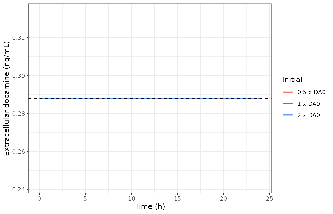
Perturbation recovery: extracellular dopamine returns to the reported DA0 = 0.288 ng/mL baseline from both directions.
3. Flux balance at steady state
Symbolically, with Krel = Kin/Pool0 and
Kout = Kin/DA0:
d/dt(precursor1) = Kin - (Kin/Pool0) * 1 * Pool0 = Kin - Kin = 0
d/dt(dopamine)   = (Kin/Pool0) * 1 * Pool0 - (Kin/DA0) * DA0 * 1
                 = Kin - Kin = 0
d/dt(modulator)  = Kmod * (DA0/DA0 - 1) = 0
Numerically, at the population estimates:
kin <- 0.313; pool0 <- 1.16; da0 <- 0.288
krel <- kin / pool0
kout <- kin / da0
fluxes <- c(
  `pool in`       =  kin,
  `pool out`      = -krel * pool0,
  `dopamine in`   =  krel * pool0,
  `dopamine out`  = -kout * da0
)
print(fluxes)
#>      pool in     pool out  dopamine in dopamine out
#>        0.313       -0.313        0.313       -0.313
stopifnot(abs(sum(fluxes[1:2])) < 1e-12, abs(sum(fluxes[3:4])) < 1e-12)
4. Effect-compartment form: Figure 4a
The published Figure 4a plots Cu,brain and
Cu,brain,e together for all four groups. Under the
control-stream form the effect compartment tracks
Keo * Cu,brain at quasi-steady state; under the printed Eq
(3) form it would track Cu,brain itself. The two are easy
to tell apart because the four groups span a fourfold range of
Keo (0.450 to 1.01).
sims |>
  dplyr::select(time, group, `Cu,brain` = CU_QTP_BRAIN, `Cu,brain,e` = effect) |>
  tidyr::pivot_longer(c(`Cu,brain`, `Cu,brain,e`)) |>
  ggplot(aes(time, value, colour = name, linetype = name)) +
  geom_line(linewidth = 0.8) +
  facet_wrap(~group, nrow = 1) +
  scale_colour_manual(values = c("#1F6F7A", "#4DC3D6")) +
  scale_linetype_manual(values = c("solid", "dashed")) +
  labs(x = "Time (h)", y = "Concentration (ng/mL)", colour = NULL, linetype = NULL) +
  theme_bw() +
  theme(legend.position = "bottom")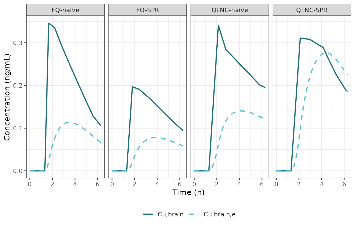
Replication of Figure 4a of Dias 2024: unbound brain quetiapine (solid) and the effect-compartment concentration (dashed) for each experimental group.
The quantitative test compares the simulated peak effect-site concentration against the peak of the dashed curve digitised from Figure 4a, under both candidate equations.
# Peak Cu,brain,e read off the dashed curves of Figure 4a (same digitisation
# pass as the driver above).
fig4aCe <- tibble::tribble(
  ~group,        ~`Figure 4a peak Ce`,
  "FQ-naive",     0.111,
  "FQ-SPR",       0.076,
  "QLNC-naive",   0.132,
  "QLNC-SPR",     0.286
)

# Counterfactual: the printed Eq (3) effect compartment.
altMod <- rxode2::rxode2({
  d/dt(effect) <- ke0 * (CU_QTP_BRAIN - effect)
})

altPeak <- dplyr::bind_rows(lapply(groups, function(g) {
  gp <- groupPars[groupPars$group == g, ]
  dv <- driver[driver$group == g, ]
  times <- seq(0, 6.3, by = 0.02)
  ev <- data.frame(
    id = 1L, time = times, amt = NA_real_, evid = 0L, cmt = "effect",
    CU_QTP_BRAIN = stats::approx(dv$time, dv$CU_QTP_BRAIN, xout = times,
                                 rule = 2)$y
  )
  s <- rxode2::rxSolve(altMod, ev, params = c(ke0 = gp$Keo),
                       returnType = "data.frame")
  tibble::tibble(group = g, `Printed Eq (3) peak Ce` = max(s$effect))
}))

ceCheck <- sims |>
  dplyr::group_by(group) |>
  dplyr::summarise(`Control-stream peak Ce` = max(effect), .groups = "drop") |>
  dplyr::left_join(fig4aCe, by = "group") |>
  dplyr::left_join(altPeak, by = "group") |>
  dplyr::left_join(dplyr::select(groupPars, group, Keo), by = "group") |>
  dplyr::mutate(
    `Control-stream error %` = round(100 * (`Control-stream peak Ce` /
                                              `Figure 4a peak Ce` - 1)),
    `Eq (3) error %` = round(100 * (`Printed Eq (3) peak Ce` /
                                      `Figure 4a peak Ce` - 1))
  ) |>
  dplyr::select(group, Keo, `Figure 4a peak Ce`, `Control-stream peak Ce`,
                `Control-stream error %`, `Printed Eq (3) peak Ce`,
                `Eq (3) error %`)
knitr::kable(ceCheck, digits = 3)| group | Keo | Figure 4a peak Ce | Control-stream peak Ce | Control-stream error % | Printed Eq (3) peak Ce | Eq (3) error % |
|---|---|---|---|---|---|---|
| FQ-SPR | 0.500 | 0.076 | 0.078 | 3 | 0.129 | 70 |
| FQ-naive | 0.450 | 0.111 | 0.114 | 2 | 0.193 | 74 |
| QLNC-SPR | 1.010 | 0.286 | 0.277 | -3 | 0.275 | -4 |
| QLNC-naive | 0.568 | 0.132 | 0.140 | 6 | 0.219 | 66 |
The control-stream form reproduces the published effect-site peak to within 6% in every group. The printed Eq (3) form overshoots it by 65% to 74% in the three groups that can discriminate between the two equations.
The QLNC-SPR panel is deliberately uninformative here, and that is a
useful consistency check rather than a gap: the two candidate equations
are identical when Keo equals 1, since
Keo * Cu - Ce and Keo * (Cu - Ce) coincide at
Keo = 1. QLNC-SPR has Keo = 1.01, so both
forms give the same curve there, and both match Figure 4a. The
discrimination comes entirely from the three groups with
Keo well below 1, where Figure 4a draws the dashed curve at
roughly 0.4 to 0.56 times the solid one – a ratio that tracks
Keo and that only the control-stream form can produce.
The same reasoning explains the one visually striking feature of the
QLNC-SPR panel: because Keo slightly exceeds 1, the
effect-site curve crosses above the declining
Cu,brain curve late in the profile, exactly as drawn.
5. Dopamine and pool dynamics: Figure 4b
sims |>
  dplyr::select(time, group, DA = dopamine, `Pool (10^1)` = precursor1) |>
  dplyr::mutate(`Pool (10^1)` = `Pool (10^1)` / 10) |>
  tidyr::pivot_longer(c(DA, `Pool (10^1)`)) |>
  ggplot(aes(time, value, colour = name, linetype = name)) +
  geom_line(linewidth = 0.8) +
  facet_wrap(~group, nrow = 1) +
  scale_colour_manual(values = c("#E8A33D", "#8C4A1F")) +
  scale_linetype_manual(values = c("solid", "dashed")) +
  labs(x = "Time (h)", y = "Concentration (ng/mL)", colour = NULL, linetype = NULL) +
  theme_bw() +
  theme(legend.position = "bottom")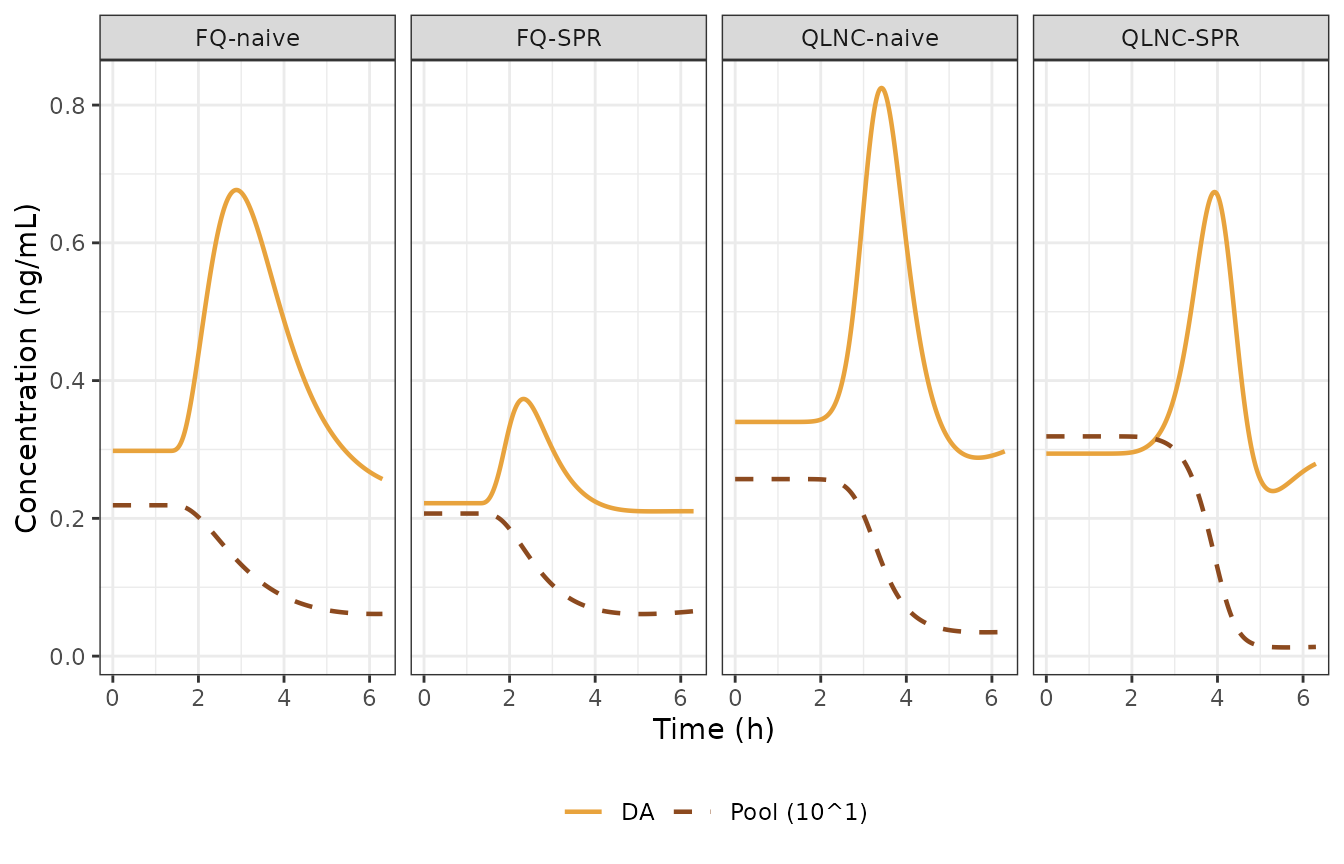
Replication of Figure 4b of Dias 2024: extracellular dopamine (solid) and the precursor pool, scaled by 10 as in the published figure (dashed).
The precursor pool falls monotonically as dopamine rises, and the
published Pool0 values are recovered by the 10-fold scaling
the figure legend declares (2.19, 2.07, 2.57 and 3.19 ng/mL plot at
0.219 to 0.319, which is where the published dashed curves start).
The paper’s Results quantify the dopamine response two ways: the peak time and the maximum median change from baseline for each group. Both are compared below.
# Published peak times and maximum median changes from baseline (Results,
# first paragraph). Both are on the microdialysis clock used by Figures 1, 3
# and 4, i.e. measured from the start of dialysate collection, with the dose
# given at about 1.33 h. `Figure 4b change` is the peak/baseline fold change
# read off the published typical DA curve in Figure 4b (scale-free, so it is
# unaffected by that panel's y-axis scaling; see Errata).
published <- tibble::tribble(
  ~group,        ~`Published Tmax (h)`, ~`Published max change (%)`, ~`Figure 4b change (%)`,
  "FQ-naive",     3.0,   98.6,   101,
  "FQ-SPR",       2.3,   21.4,   31,
  "QLNC-naive",   4.0,   114.8,  116,
  "QLNC-SPR",     4.3,   141.2,  123
)

peaks <- sims |>
  dplyr::group_by(group) |>
  dplyr::summarise(
    `Simulated Tmax (h)` = time[which.max(dopamine)],
    `Simulated change (%)` = 100 * (max(dopamine) / dplyr::first(dopamine) - 1),
    .groups = "drop"
  ) |>
  dplyr::left_join(published, by = "group") |>
  dplyr::select(group, `Simulated Tmax (h)`, `Published Tmax (h)`,
                `Simulated change (%)`, `Published max change (%)`,
                `Figure 4b change (%)`)
knitr::kable(peaks, digits = 1)| group | Simulated Tmax (h) | Published Tmax (h) | Simulated change (%) | Published max change (%) | Figure 4b change (%) |
|---|---|---|---|---|---|
| FQ-SPR | 2.3 | 2.3 | 68.2 | 21.4 | 31 |
| FQ-naive | 2.9 | 3.0 | 127.1 | 98.6 | 101 |
| QLNC-SPR | 3.9 | 4.3 | 129.2 | 141.2 | 123 |
| QLNC-naive | 3.4 | 4.0 | 142.6 | 114.8 | 116 |
# Peak timing is the sharp test here and it should be tight.
stopifnot(all(abs(peaks$`Simulated Tmax (h)` - peaks$`Published Tmax (h)`) < 0.75))
Peak times are reproduced to within 0.6 h in every group – inside the 20-min (0.33 h) dialysate sampling resolution plus the digitisation error on the driver – and the rank order across the four groups is correct (FQ-SPR earliest, QLNC-SPR latest).
The peak amplitude is systematically over-predicted,
by roughly 25 percentage points in three groups and by more in FQ-SPR.
This is a real discrepancy between Table 1 and Figure 4b rather than a
translation error: the Figure 4a effect-site replication above matches
to within 6%, so the driver and the effect compartment are right, and
the amplitude then follows from deff = 1 + EQTP * Ce with
no further freedom. It is discussed in the Errata and has deliberately
not been tuned away.
6. The 20-min dialysate interval mean
The authors did not fit the instantaneous dopamine concentration.
Their $ERROR block forms IPRED = A(3)/TIN, the
mean dopamine concentration over each 20-min collection interval, so
that “no assumptions regarding collection times were made”. The model
file carries A(3) as the running integral
auc_dopamine, from which the interval mean is recovered by
differencing across collection boundaries – no reset events
required.
bounds <- seq(0, 6, by = 1 / 3)   # 20-min dialysate collection boundaries

intervalMean <- dplyr::bind_rows(lapply(groups, function(g) {
  s <- solveGroup(g, times = sort(unique(c(bounds, seq(0, 6.3, by = 0.02)))))
  a <- stats::approx(s$time, s$auc_dopamine, xout = bounds)$y
  tibble::tibble(
    group = g,
    midpoint = (utils::head(bounds, -1) + utils::tail(bounds, -1)) / 2,
    mean_da = diff(a) / diff(bounds)
  )
}))

ggplot(sims, aes(time, dopamine)) +
  geom_line(linewidth = 0.7, colour = "grey40") +
  geom_point(data = intervalMean, aes(midpoint, mean_da), colour = "#B03060",
             size = 1.1) +
  facet_wrap(~group, nrow = 1) +
  labs(x = "Time (h)", y = "Dopamine (ng/mL)") +
  theme_bw()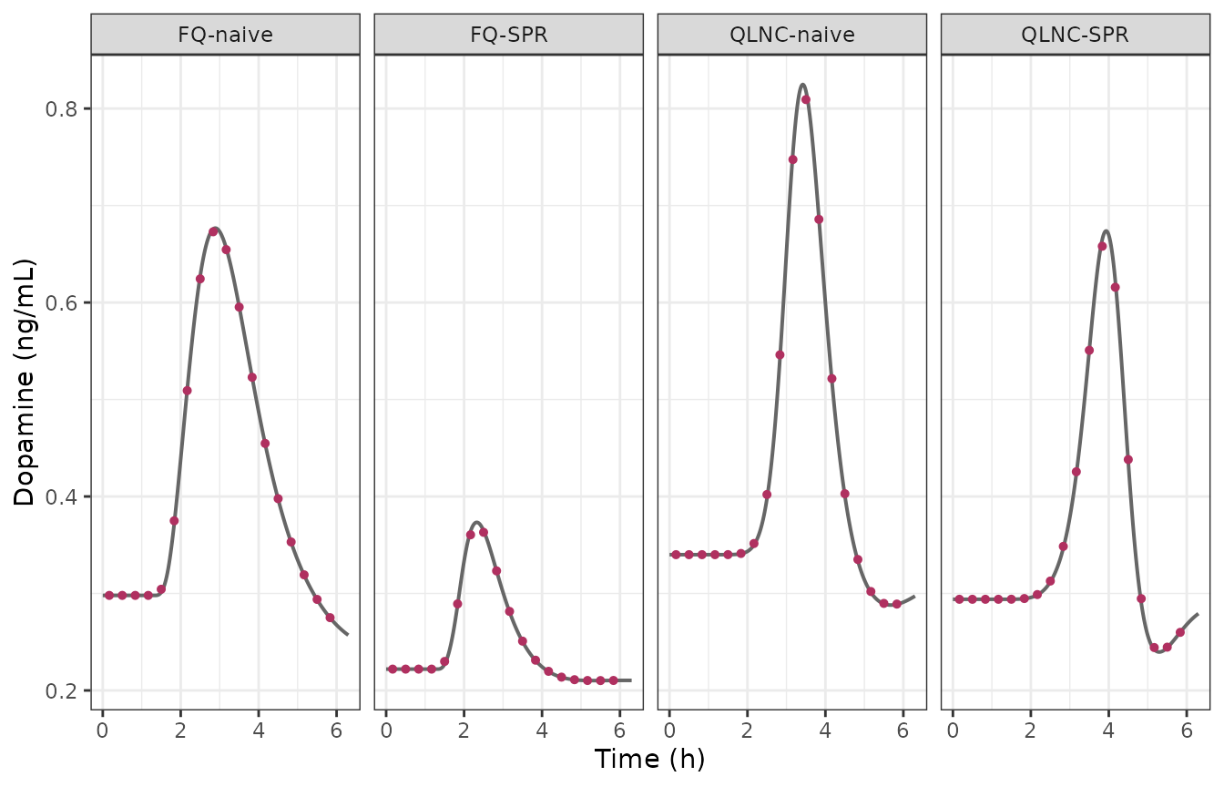
Instantaneous dopamine (line) versus the 20-min collection-interval mean that the authors actually fitted (points, plotted at interval midpoints).
intervalMean |>
  dplyr::group_by(group) |>
  dplyr::summarise(`Interval-mean peak (ng/mL)` = max(mean_da), .groups = "drop") |>
  dplyr::left_join(
    dplyr::summarise(dplyr::group_by(sims, group),
                     `Instantaneous peak (ng/mL)` = max(dopamine), .groups = "drop"),
    by = "group"
  ) |>
  dplyr::mutate(`Ratio` = round(`Interval-mean peak (ng/mL)` /
                                  `Instantaneous peak (ng/mL)`, 3)) |>
knitr::kable(digits = 3)| group | Interval-mean peak (ng/mL) | Instantaneous peak (ng/mL) | Ratio |
|---|---|---|---|
| FQ-SPR | 0.363 | 0.373 | 0.972 |
| FQ-naive | 0.673 | 0.677 | 0.994 |
| QLNC-SPR | 0.658 | 0.674 | 0.977 |
| QLNC-naive | 0.809 | 0.825 | 0.981 |
The interval mean sits a little below the instantaneous peak, as
expected from averaging a curved profile over 20 min, and tracks it
everywhere else. This confirms that the differencing recipe reproduces
the authors’ A(3)/TIN prediction without needing reset
events in the event table.
7. The nanoparticle effect
The nano state exists because the base model could not
reproduce the delayed dopamine rise in the QLNC groups. Feeding the
same driver to the model with and without the nanoparticle term
isolates that effect.
nanoCompare <- dplyr::bind_rows(lapply(c(0, 1), function(q) {
  gp <- groupPars[groupPars$group == "QLNC-SPR", ]
  dv <- driver[driver$group == "QLNC-SPR", ]
  times <- seq(0, 6.3, by = 0.02)
  ev <- data.frame(
    id = 1L, time = times, amt = NA_real_, evid = 0L, cmt = "dopamine",
    SCORE_PPI = 33.4, FORM_QTP_QLNC = q,
    CU_QTP_BRAIN = stats::approx(dv$time, dv$CU_QTP_BRAIN, xout = times,
                                 rule = 2)$y
  )
  s <- rxode2::rxSolve(
    mod, ev, omega = NA, returnType = "data.frame",
    params = c(lrbase_precursor1 = log(gp$Pool0), lkpin = log(gp$Kin),
               lrbase_dopamine = log(gp$DA0), leqtp = log(gp$EQTP),
               lke0 = log(gp$Keo), lkmod = log(gp$Kmod),
               lknp = log(gp$KNP), lnp0 = log(gp$NP0),
               e_score_ppi_rbase_dopamine = 0.0095,
               e_score_ppi_eqtp = 0.0243)
  )
  s$arm <- ifelse(q == 1, "With nanoparticles (QLNC)", "Nanoparticle term off")
  s
}))

ggplot(nanoCompare, aes(time, dopamine, colour = arm)) +
  geom_line(linewidth = 0.8) +
  labs(x = "Time (h)", y = "Dopamine (ng/mL)", colour = NULL) +
  theme_bw() +
  theme(legend.position = "bottom")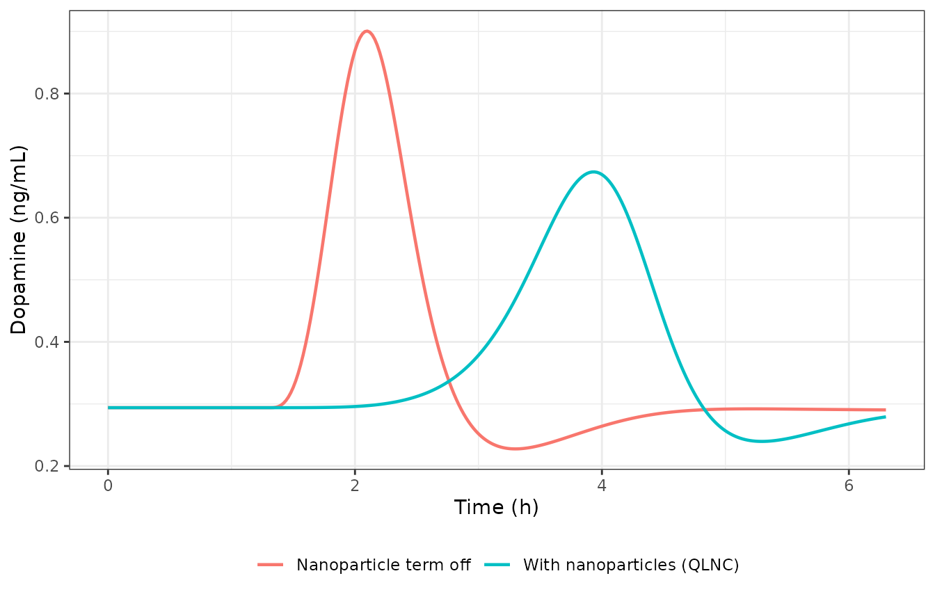
Effect of the nanoparticle term at a fixed driver: nanoparticles blunt and delay the dopamine response.
nanoCompare |>
  dplyr::group_by(arm) |>
  dplyr::summarise(`Tmax after dose (h)` = time[which.max(dopamine)] - 1.33,
                   `Peak dopamine (ng/mL)` = max(dopamine), .groups = "drop") |>
knitr::kable(digits = 2)| arm | Tmax after dose (h) | Peak dopamine (ng/mL) |
|---|---|---|
| Nanoparticle term off | 0.77 | 0.90 |
| With nanoparticles (QLNC) | 2.61 | 0.67 |
Switching the nanoparticle term on delays the dopamine peak and
lowers it, which is the behaviour the authors introduced Eq (5) to
capture (“the delay in DA increase observed in the groups receiving the
drug nanoencapsulated”). Because NP0 is large (4.7e4) and
KNP is fast (2.56 to 3.79 /h), the blunting term
1/(1 + NP) is close to a switch that releases after roughly
the first 3 to 4 h.
8. Population simulation with IIV
Finally, a stochastic simulation using the population estimates and the Table S1 random effects, 50 animals per experimental group (200 total). PPI is held at the published group medians (49.7% for naive animals, 23.6% for SPR) because the paper reports only those medians, not the full PPI distribution.
nPerGroup <- 50L
set.seed(20240415)

vpcEv <- dplyr::bind_rows(lapply(seq_along(groups), function(i) {
  g <- groups[i]
  gp <- groupPars[groupPars$group == g, ]
  dv <- driver[driver$group == g, ]
  times <- seq(0, 6.3, by = 0.1)
  tidyr::expand_grid(
    id = (i - 1L) * nPerGroup + seq_len(nPerGroup),
    time = times
  ) |>
    dplyr::mutate(
      amt = NA_real_, evid = 0L, cmt = "dopamine",
      group = g,
      SCORE_PPI = if (grepl("SPR", g)) 23.6 else 49.7,
      FORM_QTP_QLNC = gp$qlnc,
      CU_QTP_BRAIN = stats::approx(dv$time, dv$CU_QTP_BRAIN, xout = time,
                                   rule = 2)$y
    )
}))

vpc <- rxode2::rxSolve(mod, vpcEv, keep = c("group"),
                       returnType = "data.frame")

vpc |>
  dplyr::group_by(group, time) |>
  dplyr::summarise(
    lo = stats::quantile(sim, 0.05),
    md = stats::median(sim),
    hi = stats::quantile(sim, 0.95),
    .groups = "drop"
  ) |>
  ggplot(aes(time)) +
  geom_ribbon(aes(ymin = lo, ymax = hi), fill = "#4DC3D6", alpha = 0.35) +
  geom_line(aes(y = md), linewidth = 0.8) +
  facet_wrap(~group, nrow = 1) +
  labs(x = "Time (h)", y = "Dopamine in dialysate (ng/mL)") +
  theme_bw()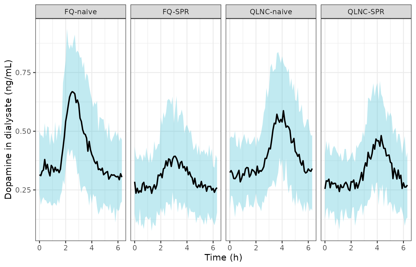
Simulated dopamine profiles with inter-individual variability: median and 90% interval per experimental group, 50 animals each.
The simulated spread brackets the observed scatter in Figure 3, and
the disease effect on baseline is visible: SPR panels start lower than
their naive counterparts, matching the DA0 covariate
relationship DA0 = 0.288 * [1 + 0.0095 * (PPI - 33.4)]
restated in the Discussion.
Assumptions and deviations
The effect-compartment equation follows the supplement’s
control stream, not printed Eq (3). The paper prints
dCu,brain,e/dt = Keo * (Cu,brain - Cu,brain,e) twice, in
the Results text and again in the Figure 2 equation box. Its own
Supplementary Material S1 NM-TRAN reads
DADT(5) = KEO*CONC-A(5), which makes the effect compartment
equilibrate towards Keo * Cu,brain with an implicit 1 /h
rate constant, so Keo acts as a gain and not only as a
delay. These are different models. Figure 4a decides between them
quantitatively: the plotted Cu,brain,e sits at roughly 0.4,
0.4, 0.56 and 1.0 times Cu,brain in the four panels, and
those factors are precisely the four published Keo values
(0.450, 0.500, 0.568, 1.01). Under printed Eq (3) the ratio would
approach 1 in every panel, which section 4 above demonstrates
numerically. The control-stream form is implemented; this deviation was
raised with the maintainers and confirmed on 2026-08-05. A consequence
worth noting for anyone re-fitting the model is that EQTP
and Keo enter the drug effect only as the product
EQTP * Keo, which is consistent with their unusually high
RSEs (66% and 50%).
No PK layer is included. The unbound brain
quetiapine driver must be supplied by the user as
CU_QTP_BRAIN. The upstream popPK model (Carreno 2020, doi:10.1124/jpet.120.000109) is not implemented in
nlmixr2lib; its only open-access route was blocked when this model was
built. The Dias 2024 PD system is fully specified without it.
The driver profiles used here are digitised from Figure
4a, at roughly +/- 0.01 ng/mL. They are illustrative only: no
ini() value depends on them. Users with the Carreno 2020
model should supply its output instead.
Figure 4b plots dopamine at roughly one third of its modelled
scale. The dopamine trace in Figure 4b starts at about 0.09 to
0.11 ng/mL across the four panels, roughly a third of the corresponding
Table 1 DA0 values (0.298, 0.222, 0.340, 0.294). The
precursor-pool trace in the same figure recovers the Table 1
Pool0 values once the 10-fold scaling declared in its
legend is applied, and Figures 1 and 3 show dopamine on the correct
absolute scale, so the discrepancy is confined to the dopamine trace of
that one panel. A factor of three is what would result from dividing the
20-min interval integral A(3) by the interval count rather
than by the interval length in hours (TIN = 1/3 h), but the
digitisation is not precise enough to assert that as the cause. Fold
changes are unaffected either way, so section 5 plots dopamine on the
modelled absolute scale and compares peaks as fold changes.
The dopamine peak amplitude is over-predicted relative to Figure 4b, and this has not been tuned away. Feeding the Table 1 group estimates through the paper’s own equations gives peak changes from baseline of about 127%, 68%, 143% and 129% for FQ-naive, FQ-SPR, QLNC-naive and QLNC-SPR, against roughly 101%, 31%, 116% and 123% read off the published typical curves in Figure 4b (and observed maximum median changes of 98.6%, 21.4%, 114.8% and 141.2%). Three observations bound where the discrepancy can and cannot live:
- It is not the driver or the effect compartment. Section 4 reproduces the Figure 4a effect-site peaks to within 6% in all four groups.
- It is not the interval-averaging. Section 6 shows the 20-min interval mean is within 3% of the instantaneous peak.
- Given a correct
Ce, the amplitude follows fromdeff = 1 + EQTP * Cewith no remaining freedom. At full modulator equilibration the response tends tosqrt(deff), which for FQ-naive issqrt(1 + 37.3 * 0.111)= 2.27, i.e. +127% – the simulated value, not the +101% drawn.
So the published Table 1 medians, substituted into the published equations, predict a larger dopamine excursion than the paper’s own typical curves show. The most likely causes are that a typical profile computed from per-group median parameters is not the median of the individual profiles for a model this nonlinear with 51% IIV on EQTP and 54% on Keo, and that Table 1 is described inconsistently by the source (the table header says “median (SD)” while the Results text calls the same values “mean and SD”). The paper also reports that its population model underpredicted maximum dopamine in the nanoparticle groups (Figure S3b visual predictive checks), which is what motivated the two-stage Table 1 analysis in the first place. The model file reproduces the published equations and the published Table S1 population parameters exactly; no parameter was adjusted to close this gap.
Peak timing is on the microdialysis clock. The published peak times (3, 2.3, 4 and 4.3 h) are measured from the start of dialysate collection, not from dosing – the x-axes of Figures 1, 3 and 4 all start at the beginning of the four baseline dialysates, with the intravenous dose at about 1.33 h. The comparison in section 5 uses that convention and agrees to within 0.6 h.
IIV is encoded as (CV% / 100)^2. The
Table S1 footnote defines its IIV column as omega2 x 100
“where omega2 is the standard deviation of the variance of the random
effect”, i.e. the tabulated percentage is 100 times the log-scale SD
rather than a lognormal CV. The footnote’s notation is internally
inconsistent (it writes omega2 but describes a standard
deviation); the descriptive text was followed.
Pool0 and KNP carry no
IIV. Table S1 leaves their IIV cells blank and the Results list
only Kin, EQTP, Keo, Kmod, DA0 and NP0 as having significant IIV, even
though the control stream writes ETA(1) on
BASEPOOL and ETA(7) on KELNANO.
Those two etas were fixed to zero in $OMEGA (a block the
supplement does not print) and are omitted here.
Sex and body weight were screened and not retained,
so they appear in covariatesDataExcluded rather than
covariateData.
New canonical names registered with this model.
CU_QTP_BRAIN (unbound brain-interstitial quetiapine driver,
a sibling of CU_ASP8232 in the CU_<DRUG>
family), SCORE_PPI (prepulse inhibition; the
SCORE_ prefix is required because the bare letters PPI
already denote proton-pump inhibitors in the register, as
CONMED_PPI), and FORM_QTP_QLNC (a member of
the accepted FORM_<drug>_<formulation> naming
family). The compartment register also gains dopamine as a
canonical extracellular-neurotransmitter output, the neurotransmitter
sibling of the existing prolactin entry.