Trimethoprim + sulfadiazine / sulfadimethoxine / sulfamethoxazole in pigs (Boulanger 2025) • nlmixr2lib

mod <- rxode2::rxode(readModelDb("Boulanger_2025_trimethoprim_sulfonamides_pig"))
#> ℹ parameter labels from comments will be replaced by 'label()'
#> Warning: some etas defaulted to non-mu referenced, possible parsing error: etaiov_cl_sdz_1, etaiov_cl_1, etaiov_vc_sdmx_1, etaiov_vc_1, etaiov_vp_sdmx_1, etaiov_vp_sdz_1, etaiov_vp_1, etaiov_cl_sdz_2, etaiov_cl_2, etaiov_vc_sdmx_2, etaiov_vc_2, etaiov_vp_sdmx_2, etaiov_vp_sdz_2, etaiov_vp_2, etaiov_cl_sdz_3, etaiov_cl_3, etaiov_vc_sdmx_3, etaiov_vc_3, etaiov_vp_sdmx_3, etaiov_vp_sdz_3, etaiov_vp_3, etaiov_cl_sdmx_1, etaiov_cl_sdmx_2, etaiov_cl_sdmx_3, etaiov_vc_sdz_1, etaiov_vc_sdz_2, etaiov_vc_sdz_3, etaiov_vc_smx_1, etaiov_vc_smx_2, etaiov_vc_smx_3, etaiov_vp_smx_1, etaiov_vp_smx_2, etaiov_vp_smx_3
#> as a work-around try putting the mu-referenced expression on a simple line

Model and source

Citation: Boulanger M, Taillandier JF, Henri J, Devreese M, De Baere S, Lacroix M, Ferran AA, Viel A. Population pharmacokinetic modeling of sulfadimethoxine, sulfadiazine and sulfamethoxazole combined to trimethoprim in pigs. Vet Q. 2025;45(1):1-17. doi:10.1080/01652176.2025.2565351. Fixed effects, random-effect standard deviations and residual error from Table 2; random-effect correlations from Supplementary Table S6; protein binding from the Results ‘Protein binding experiment’ section.
Article: https://doi.org/10.1080/01652176.2025.2565351
Supplement (Tables S1-S6): https://www.ebi.ac.uk/europepmc/webservices/rest/PMC12481524/supplementaryFiles

Sulfonamides are combined with trimethoprim (TMP) in a fixed 1:5 TMP:sulfonamide dose ratio in essentially every veterinary formulation, on the assumption that this reproduces the 1:19 in vivo concentration ratio considered optimal for synergy in human medicine. Boulanger and colleagues ran three cross-over PK studies in growing pigs – one per licensed combination – and fitted all four drugs simultaneously in Monolix to test that assumption.

The headline result is that the 1:19 target is essentially never met: at the marketed doses only 8.8% (TMP/SMX), 46.8% (TMP/SDZ) and 76.5% (TMP/SDMX) of simulated pigs fall inside even a relaxed 1:10-1:50 window.

Why this is one model file and not four

The paper states that “a structural model was developed for each drug estimating its own structural parameters”, which reads like four independent models. It is not. Supplementary Table S6 reports 21 random-effect correlations, and those correlations are cross-drug – CL_TMP - CL_SDZ, V1_SDMX - CL_SDZ, V2_TMP - V1_SDMX, and so on. Twenty-one is exactly the number of off-diagonal pairs in a 7x7 matrix, and the seven random effects involved (CL_SDZ, CL_TMP, V1_SDMX, V1_TMP, V2_SDMX, V2_SDZ, V2_TMP) span three of the four drugs. So the four structural sub-models share a single variance-covariance matrix and are one statistical model.

That matters for use, not just for bookkeeping: the paper’s central output is the ratio of TMP to sulfonamide concentration in the same animal, and the authors say explicitly that the correlations are “important for the simulating a large cohort of individuals to avoid unrealistic variability”. Splitting the extraction into four files would silently discard them and inflate the spread of the simulated ratio. The model is therefore packaged as one file, with TMP holding the unsuffixed canonical names and the sulfonamides carrying the sibling-drug suffixes _sdz, _sdmx and _smx.

mod$state
#>  [1] "depot"            "depot2"           "central"          "peripheral1"     
#>  [5] "depot_sdz"        "depot2_sdz"       "central_sdz"      "peripheral1_sdz" 
#>  [9] "depot_sdmx"       "central_sdmx"     "peripheral1_sdmx" "depot_smx"       
#> [13] "central_smx"      "peripheral1_smx"

Population

pop <- mod$population
str(pop, max.level = 1, give.attr = FALSE)
#> List of 11
#>  $ species       : chr "pig (Large White x Landrace)"
#>  $ n_subjects    : num 34
#>  $ n_studies     : num 4
#>  $ age_range     : chr "7-8 weeks at enrolment"
#>  $ weight_range  : chr "23.8-46.8 kg"
#>  $ weight_median : chr "31.1 kg"
#>  $ sex_female_pct: num 100
#>  $ disease_state : chr "healthy growing pigs"
#>  $ dose_range    : chr "single dose of licensed 1:5 TMP:S products - TMP/SDZ 2.5+12.5 mg/kg IV and IM, 5+25 mg/kg oral; TMP/SDMX 4+18.6"| __truncated__
#>  $ regions       : chr "France and Belgium"
#>  $ notes         : chr "Three independent two-period cross-over studies with 10 (TMP/SDZ), 10 (TMP/SMX) and 14 (TMP/SDMX) pigs; all ani"| __truncated__

Thirty-four healthy female Large White x Landrace pigs, 7-8 weeks old at enrolment, weighing 23.8-46.8 kg (median 31.1 kg), took part in three independent two-period cross-over studies: 10 pigs on TMP/SDZ, 10 on TMP/SMX and 14 on TMP/SDMX (Table 1). Each pig received the combination intravenously in one period and orally in the other; eight of the TMP/SDZ pigs received an additional intramuscular dose in a third period. Individual raw data from De Smet et al. (2017) – multiple-dose oral and intramuscular SDZ/TMP – were pooled in to support the SDZ and TMP sub-models, giving four contributing studies in total. Of the 1858 concentrations included in the modelling, 155 were considered outliers, as were three animals (one on TMP/SDMX, two on TMP/SMX), mainly because of catheter problems; SMX concentrations beyond 12 h were discarded because the assay returned implausibly flat values (Results, “PK data after administration”).

Mean in vivo plasma protein binding, measured by ultrafiltration in a subset of pigs after IV dosing, was 29.2% for SDZ, 57.3% for SMX, 94.1% for SDMX and 51.2% for TMP – unbound fractions of 0.708, 0.427, 0.059 and 0.489 respectively (Results, “Protein binding experiment”). These are used below to convert the simulated total concentrations to the free concentrations that drive the ratio.

Source trace

Every ini() entry in inst/modeldb/specificDrugs/Boulanger_2025_trimethoprim_sulfonamides_pig.R carries an in-file comment naming its origin. Collected here:

Equation / parameter	Value	Source location
Two-compartment disposition, each drug	–	Results, “Population PK analysis” (BICc + GOF selection)
Individual-parameter model with IIV + IOV	–	Methods Equation 2
Body-weight power model, normalised to 31.1 kg	–	Methods Equation 3
`lka` / `lka_sdz` / `lka_sdmx` / `lka_smx`	0.66 / 0.50 / 0.60 / 1.82 1/h	Table 2, `ka_TMP` / `ka_SDZ` / `ka_SDMX` / `ka_SMX`
`lka2` / `lka2_sdz` (intramuscular)	1.14 / 1.3 1/h	Table 2, `ka_TMP_IM` / `ka_SDZ_IM`
`lfdepot` / `lfdepot_sdz` / `lfdepot_sdmx` / `lfdepot_smx`	0.58 / 0.93 / 0.68 / 0.64	Table 2, `F_*_oral`
`lfdepot2` / `lfdepot2_sdz` (intramuscular)	0.99 / 0.99	Table 2, `F_TMP_IM` / `F_SDZ_IM`
`lcl` / `lcl_sdz` / `lcl_sdmx` / `lcl_smx`	0.48 / 0.12 / 0.015 / 0.21 L/h/kg	Table 2, `Cl_*`
`lvc` / `lvc_sdz` / `lvc_sdmx` / `lvc_smx`	0.92 / 0.3 / 0.13 / 0.48 L/kg	Table 2, `V1_*`
`lq` / `lq_sdz` / `lq_sdmx` / `lq_smx`	1.26 / 0.32 / 0.20 / 0.83 L/h/kg	Table 2, `Q_*`
`lvp` / `lvp_sdz` / `lvp_sdmx` / `lvp_smx`	0.86 / 0.29 / 0.16 / 0.17 L/kg	Table 2, `V2_*`
`e_wt_cl` / `e_wt_vc`	0.78 / 1.33	Table 2, `beta_Cl_TMP_BW` / `beta_V1_TMP_BW`
`e_wt_cl_sdz` / `e_wt_vc_sdz`	0.51 / 1.1	Table 2, `beta_Cl_SDZ_BW` / `beta_V1_SDZ_BW`
`etalka` / `etalka_sdz` / `etalka_sdmx`	0.63 / 0.52 / 0.37 (SD)	Table 2, `omega_ka_*`, squared to variance
IOV SDs on CL, V1, V2	0.09-0.62 (SD)	Table 2, `gamma_*`, squared to variance
IOV correlations (7x7 block)	21 pairwise values	Supplementary Table S6
`expSd` / `expSd_sdz` / `expSd_sdmx` / `expSd_smx`	0.40 / 0.32 / 0.22 / 0.18	Table 2, `a_*` (constant error on log-transformed concentrations)
Unbound fractions 0.489 / 0.708 / 0.059 / 0.427	–	Results, “Protein binding experiment”
Doses per route and combination	–	Table 1
Reference NCA values (t1/2, AUCinf)	–	Table 3

Two points about the parameterisation are worth stating explicitly, because they are implicit in the paper rather than written out.

Everything is per kilogram. Table 1 gives every dose in mg/kg, and Table 2 reports clearances in L/h/kg and volumes in L/kg. Feeding a mg/kg amount into an L/kg volume gives mg/L = ug/mL directly, which is the unit of the reported concentrations. The model therefore expects amt in mg/kg and needs no separate weight-scaling of the dose.

Equation 3 is a power model. Both structural equations are printed on page 7 of the article:

Log(H_ik) = log(H_pop) + eta_Hi + gamma_Hi                          (Eq 2)
Log(H_i)  = log(H_pop) + beta_BW x log(BW / 31.1) + eta_Hi + gamma_Hik  (Eq 3)

Adding beta_BW * log(BW/31.1) on the log scale is multiplying by (BW/31.1)^beta_BW on the natural scale, so Equation 3 is a power model normalised to the 31.1 kg median pig, and Equation 2 puts both random effects additively on the log scale – i.e. log-normal IIV and IOV, exactly as encoded. The Discussion independently supplies four worked examples that confirm the reading – see the covariate check below.

Checking Equation 3 against the Discussion

The Discussion states that for a 41.1 kg pig (10 kg above the 31.1 kg median), CL rises from 0.12 to 0.14 L/h/kg (SDZ) and 0.48 to 0.60 L/h/kg (TMP), and V1 from 0.30 to 0.41 L/kg (SDZ) and 0.92 to 1.33 L/kg (TMP). A power model P = P_pop * (BW/31.1)^beta reproduces all four:

cov_probe <- function(wt) {
  ev <- rbind(
    data.frame(time = 0, amt = 1, cmt = "central", evid = 1L, dvid = NA_integer_),
    data.frame(time = 1, amt = NA_real_, cmt = NA_character_, evid = 0L, dvid = 1L)
  ) |>
    dplyr::mutate(id = 1L, WT = wt, OCC = 1L)
  s <- rxode2::rxSolve(rxode2::zeroRe(mod), ev, returnType = "data.frame",
                       useLinCmt = FALSE)
  c(CL_TMP = s$cl[1], V1_TMP = s$vc[1], CL_SDZ = s$cl_sdz[1], V1_SDZ = s$vc_sdz[1])
}

covariate_check <- tibble::tibble(
  Parameter   = c("CL_TMP (L/h/kg)", "V1_TMP (L/kg)", "CL_SDZ (L/h/kg)", "V1_SDZ (L/kg)"),
  `Model 31.1 kg` = round(cov_probe(31.1), 3),
  `Paper 31.1 kg` = c(0.48, 0.92, 0.12, 0.30),
  `Model 41.1 kg` = round(cov_probe(41.1), 3),
  `Paper 41.1 kg` = c(0.60, 1.33, 0.14, 0.41)
)
#> Warning: some etas defaulted to non-mu referenced, possible parsing error: etaiov_cl_sdz_1, etaiov_cl_1, etaiov_vc_sdmx_1, etaiov_vc_1, etaiov_vp_sdmx_1, etaiov_vp_sdz_1, etaiov_vp_1, etaiov_cl_sdz_2, etaiov_cl_2, etaiov_vc_sdmx_2, etaiov_vc_2, etaiov_vp_sdmx_2, etaiov_vp_sdz_2, etaiov_vp_2, etaiov_cl_sdz_3, etaiov_cl_3, etaiov_vc_sdmx_3, etaiov_vc_3, etaiov_vp_sdmx_3, etaiov_vp_sdz_3, etaiov_vp_3, etaiov_cl_sdmx_1, etaiov_cl_sdmx_2, etaiov_cl_sdmx_3, etaiov_vc_sdz_1, etaiov_vc_sdz_2, etaiov_vc_sdz_3, etaiov_vc_smx_1, etaiov_vc_smx_2, etaiov_vc_smx_3, etaiov_vp_smx_1, etaiov_vp_smx_2, etaiov_vp_smx_3
#> as a work-around try putting the mu-referenced expression on a simple line
#> ℹ omega/sigma items treated as zero: 'etalka', 'etalka_sdz', 'etalka_sdmx', 'etaiov_cl_sdz_1', 'etaiov_cl_1', 'etaiov_vc_sdmx_1', 'etaiov_vc_1', 'etaiov_vp_sdmx_1', 'etaiov_vp_sdz_1', 'etaiov_vp_1', 'etaiov_cl_sdz_2', 'etaiov_cl_2', 'etaiov_vc_sdmx_2', 'etaiov_vc_2', 'etaiov_vp_sdmx_2', 'etaiov_vp_sdz_2', 'etaiov_vp_2', 'etaiov_cl_sdz_3', 'etaiov_cl_3', 'etaiov_vc_sdmx_3', 'etaiov_vc_3', 'etaiov_vp_sdmx_3', 'etaiov_vp_sdz_3', 'etaiov_vp_3', 'etaiov_cl_sdmx_1', 'etaiov_cl_sdmx_2', 'etaiov_cl_sdmx_3', 'etaiov_vc_sdz_1', 'etaiov_vc_sdz_2', 'etaiov_vc_sdz_3', 'etaiov_vc_smx_1', 'etaiov_vc_smx_2', 'etaiov_vc_smx_3', 'etaiov_vp_smx_1', 'etaiov_vp_smx_2', 'etaiov_vp_smx_3'
#> Warning: some etas defaulted to non-mu referenced, possible parsing error: etaiov_cl_sdz_1, etaiov_cl_1, etaiov_vc_sdmx_1, etaiov_vc_1, etaiov_vp_sdmx_1, etaiov_vp_sdz_1, etaiov_vp_1, etaiov_cl_sdz_2, etaiov_cl_2, etaiov_vc_sdmx_2, etaiov_vc_2, etaiov_vp_sdmx_2, etaiov_vp_sdz_2, etaiov_vp_2, etaiov_cl_sdz_3, etaiov_cl_3, etaiov_vc_sdmx_3, etaiov_vc_3, etaiov_vp_sdmx_3, etaiov_vp_sdz_3, etaiov_vp_3, etaiov_cl_sdmx_1, etaiov_cl_sdmx_2, etaiov_cl_sdmx_3, etaiov_vc_sdz_1, etaiov_vc_sdz_2, etaiov_vc_sdz_3, etaiov_vc_smx_1, etaiov_vc_smx_2, etaiov_vc_smx_3, etaiov_vp_smx_1, etaiov_vp_smx_2, etaiov_vp_smx_3
#> as a work-around try putting the mu-referenced expression on a simple line
#> ℹ omega/sigma items treated as zero: 'etalka', 'etalka_sdz', 'etalka_sdmx', 'etaiov_cl_sdz_1', 'etaiov_cl_1', 'etaiov_vc_sdmx_1', 'etaiov_vc_1', 'etaiov_vp_sdmx_1', 'etaiov_vp_sdz_1', 'etaiov_vp_1', 'etaiov_cl_sdz_2', 'etaiov_cl_2', 'etaiov_vc_sdmx_2', 'etaiov_vc_2', 'etaiov_vp_sdmx_2', 'etaiov_vp_sdz_2', 'etaiov_vp_2', 'etaiov_cl_sdz_3', 'etaiov_cl_3', 'etaiov_vc_sdmx_3', 'etaiov_vc_3', 'etaiov_vp_sdmx_3', 'etaiov_vp_sdz_3', 'etaiov_vp_3', 'etaiov_cl_sdmx_1', 'etaiov_cl_sdmx_2', 'etaiov_cl_sdmx_3', 'etaiov_vc_sdz_1', 'etaiov_vc_sdz_2', 'etaiov_vc_sdz_3', 'etaiov_vc_smx_1', 'etaiov_vc_smx_2', 'etaiov_vc_smx_3', 'etaiov_vp_smx_1', 'etaiov_vp_smx_2', 'etaiov_vp_smx_3'
knitr::kable(covariate_check, caption = "Body-weight covariate model against the four worked examples in the Discussion of Boulanger 2025.")

Body-weight covariate model against the four worked examples in the Discussion of Boulanger 2025.
Parameter	Model 31.1 kg	Paper 31.1 kg	Model 41.1 kg	Paper 41.1 kg
CL_TMP (L/h/kg)	0.48	0.48	0.597	0.60
V1_TMP (L/kg)	0.92	0.92	1.333	1.33
CL_SDZ (L/h/kg)	0.12	0.12	0.138	0.14
V1_SDZ (L/kg)	0.30	0.30	0.408	0.41

All four agree to the paper’s stated precision, confirming both the power form and the 31.1 kg normalisation constant.

Study design

# Table 1: single doses of the licensed 1:5 TMP:S products.
design <- tibble::tribble(
  ~combo,      ~sulfa,  ~admin, ~amt_tmp, ~amt_s, ~cmt_tmp,  ~cmt_s,        ~n_pigs, ~wt_lo, ~wt_hi,
  "TMP/SDZ",   "SDZ",   "IV",       2.5,   12.5,  "central", "central_sdz",      10,   28.0,   46.8,
  "TMP/SDZ",   "SDZ",   "Oral",     5.0,   25.0,  "depot",   "depot_sdz",        10,   28.0,   46.8,
  "TMP/SDZ",   "SDZ",   "IM",       2.5,   12.5,  "depot2",  "depot2_sdz",        8,   28.0,   46.8,
  "TMP/SDMX",  "SDMX",  "IV",       4.0,   18.6,  "central", "central_sdmx",     14,   23.8,   43.6,
  "TMP/SDMX",  "SDMX",  "Oral",     8.0,   37.36, "depot",   "depot_sdmx",       14,   23.8,   43.6,
  "TMP/SMX",   "SMX",   "IV",       6.0,   30.0,  "central", "central_smx",      10,   28.3,   37.2,
  "TMP/SMX",   "SMX",   "Oral",     6.0,   30.0,  "depot",   "depot_smx",        10,   28.3,   37.2
)
# Occasion assignment. In Table 1 the cross-over means each route appears in
# BOTH occasion 1 and occasion 2 (e.g. TMP/SDZ IV is 4 pigs in occ.1 plus 4 in
# occ.2), and occasion 3 is the extra intramuscular period given to 8 TMP/SDZ
# pigs. Here each route is pinned to one occasion slot purely so every arm
# draws an IOV realisation; because Table 2 reports a single IOV magnitude per
# parameter, the three slots are numerically interchangeable and the choice has
# no effect on any result below.
design$occ <- ifelse(design$admin == "IM", 3L, ifelse(design$admin == "IV", 1L, 2L))
knitr::kable(design[, c("combo", "admin", "amt_tmp", "amt_s", "n_pigs", "wt_lo", "wt_hi", "occ")],
             caption = "Single-dose design from Table 1 of Boulanger 2025 (doses in mg/kg); the occasion column is the simulation's assignment, not a column of Table 1.")

Single-dose design from Table 1 of Boulanger 2025 (doses in mg/kg); the occasion column is the simulation’s assignment, not a column of Table 1.
combo	admin	amt_tmp	amt_s	n_pigs	wt_lo	wt_hi	occ
TMP/SDZ	IV	2.5	12.50	10	28.0	46.8	1
TMP/SDZ	Oral	5.0	25.00	10	28.0	46.8	2
TMP/SDZ	IM	2.5	12.50	8	28.0	46.8	3
TMP/SDMX	IV	4.0	18.60	14	23.8	43.6	1
TMP/SDMX	Oral	8.0	37.36	14	23.8	43.6	2
TMP/SMX	IV	6.0	30.00	10	28.3	37.2	1
TMP/SMX	Oral	6.0	30.00	10	28.3	37.2	2

Virtual cohort and simulation

Each arm gets 100 pigs – more than the 8-14 actually studied, enough to stabilise the summary statistics, and well inside the 200-per-arm cap for a validation vignette. Body weights are drawn uniformly across the range reported for that combination.

n_per_arm <- 100L
obs_end   <- c(SDZ = 48, SDMX = 168, SMX = 48)   # long enough for AUCinf on each sulfonamide

simulate_arm <- function(row) {
  tmax <- obs_end[[row$sulfa]]
  grid <- sort(unique(c(seq(0, 6, by = 0.1), seq(6, 24, by = 0.5), seq(24, tmax, by = 2))))
  ids  <- seq_len(n_per_arm)
  wt   <- stats::runif(n_per_arm, row$wt_lo, row$wt_hi)

  dose <- tidyr::expand_grid(id = ids, k = 1:2) |>
    dplyr::mutate(
      time = 0,
      amt  = ifelse(k == 1, row$amt_tmp, row$amt_s),
      cmt  = ifelse(k == 1, row$cmt_tmp, row$cmt_s),
      evid = 1L, dvid = NA_integer_
    ) |>
    dplyr::select(-k)
  obs <- tidyr::expand_grid(id = ids, time = grid) |>
    dplyr::mutate(amt = NA_real_, cmt = NA_character_, evid = 0L, dvid = 1L)

  ev <- dplyr::bind_rows(dose, obs) |>
    dplyr::arrange(id, time, dplyr::desc(evid)) |>
    dplyr::mutate(WT = wt[id], OCC = row$occ)

  # dvid alone on observation rows: this model declares four endpoints, so a
  # bare ODE-state cmt cannot identify which endpoint an observation belongs
  # to. useLinCmt = FALSE keeps the auto ODE -> linCmt conversion from
  # corrupting the dvid mapping.
  rxode2::rxSolve(mod, ev, keep = c("WT", "OCC"), returnType = "data.frame",
                  useLinCmt = FALSE) |>
    dplyr::mutate(combo = row$combo, sulfa = row$sulfa, admin = row$admin)
}

sim <- dplyr::bind_rows(lapply(seq_len(nrow(design)), \(i) simulate_arm(design[i, ])))
nrow(sim)
#> [1] 88300

Cc, Cc_sdz, Cc_sdmx and Cc_smx are the individual predictions; residual error lives in the sim column and is deliberately not used here, because the paper’s Table 3 reports secondary parameters derived from the individual model fits rather than from noisy observations.

# Collapse the four analyte columns down to the two that are dosed in each arm.
long <- sim |>
  dplyr::mutate(
    conc_s = dplyr::case_when(
      sulfa == "SDZ"  ~ Cc_sdz,
      sulfa == "SDMX" ~ Cc_sdmx,
      sulfa == "SMX"  ~ Cc_smx
    )
  ) |>
  dplyr::select(id, time, combo, sulfa, admin, WT, TMP = Cc, S = conc_s) |>
  tidyr::pivot_longer(c(TMP, S), names_to = "which", values_to = "conc") |>
  dplyr::mutate(analyte = ifelse(which == "TMP", "TMP", sulfa))

Concentration-time profiles

prof <- long |>
  dplyr::filter(time <= 48) |>
  dplyr::group_by(analyte, admin, time) |>
  dplyr::summarise(med = stats::median(conc), lo = stats::quantile(conc, 0.05),
                   hi = stats::quantile(conc, 0.95), .groups = "drop") |>
  dplyr::filter(med > 0)

ggplot(prof, aes(time, med, colour = admin, fill = admin)) +
  geom_ribbon(aes(ymin = lo, ymax = hi), alpha = 0.15, colour = NA) +
  geom_line(linewidth = 0.7) +
  facet_wrap(~analyte, scales = "free_y") +
  scale_y_log10() +
  labs(x = "Time (h)", y = "Total plasma concentration (ug/mL)",
       colour = "Route", fill = "Route") +
  theme_bw()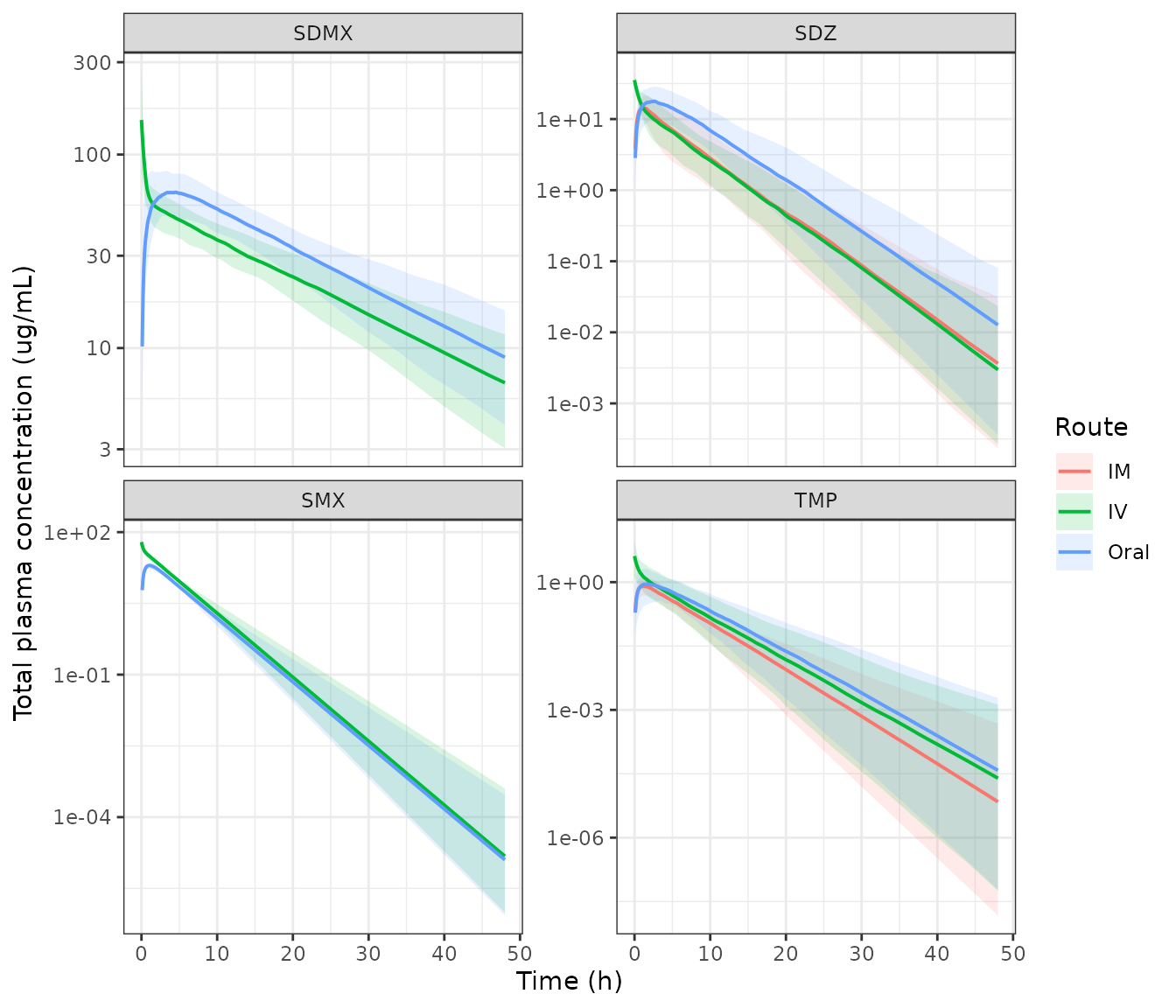

Simulated median (line) and 5th-95th percentile (band) total plasma concentrations by analyte and route. Compare with Figure 1 of Boulanger 2025.

PKNCA validation

The observation grid runs to 168 h in the TMP/SDMX arms so that sulfadimethoxine (14.8 h half-life) is followed far enough for aucinf.obs. Trimethoprim, with a 2.9 h half-life, is long gone by then – its simulated concentration underflows to zero well before the end of that grid, which leaves lambda_z fitted on numerical dust and returns NA for both half-life and AUCinf.

The fix is the one the analytical method already imposes: truncate each analyte’s NCA input at its own limit of quantification. Figure 1 of the paper gives them as 0.01 ug/mL for TMP, 0.1 ug/mL for SDZ and SDMX, and 0.02 ug/mL for SMX. The time-zero record is kept unconditionally, as PKNCA requires.

# Limits of quantification, Figure 1 caption of Boulanger 2025 (ug/mL).
loq <- c(TMP = 0.01, SDZ = 0.1, SDMX = 0.1, SMX = 0.02)

# PKNCA reserves the column names `dose` and `route`, hence `dosemgkg` / `admin`.
nca_conc <- long |>
  dplyr::filter(!is.na(conc)) |>
  dplyr::filter(time == 0 | conc >= loq[analyte])

nca_dose <- design |>
  dplyr::select(combo, admin, amt_tmp, amt_s, sulfa) |>
  tidyr::pivot_longer(c(amt_tmp, amt_s), names_to = "which", values_to = "dosemgkg") |>
  dplyr::mutate(analyte = ifelse(which == "amt_tmp", "TMP", sulfa)) |>
  dplyr::select(combo, admin, analyte, dosemgkg) |>
  tidyr::expand_grid(id = seq_len(n_per_arm)) |>
  dplyr::mutate(time = 0)

o_conc <- PKNCA::PKNCAconc(nca_conc, conc ~ time | combo + admin + analyte + id)
o_dose <- PKNCA::PKNCAdose(nca_dose, dosemgkg ~ time | combo + admin + analyte + id)

intervals <- data.frame(
  start = 0, end = Inf,
  cmax = TRUE, tmax = TRUE, half.life = TRUE,
  aucinf.obs = TRUE, auclast = TRUE, cl.obs = TRUE
)

res <- PKNCA::pk.nca(PKNCA::PKNCAdata(o_conc, o_dose, intervals = intervals))
nca <- as.data.frame(res)
head(nca, 3)
#> # A tibble: 3 × 9
#>   combo    admin analyte    id start   end PPTESTCD PPORRES exclude
#>   <chr>    <chr> <chr>   <int> <dbl> <dbl> <chr>      <dbl> <chr>  
#> 1 TMP/SDMX IV    SDMX        1     0   Inf auclast   1455.  <NA>   
#> 2 TMP/SDMX IV    SDMX        1     0   Inf cmax        94.2 <NA>   
#> 3 TMP/SDMX IV    SDMX        1     0   Inf tmax         0   <NA>

Structural identity: AUCinf must equal F x Dose / CL

For a linear model this is exact, so it is a sharp test of the whole chain – parameterisation, unit convention, bioavailability target and dose bookkeeping. It is checked per subject, not on a median.

fvals <- c(TMP_Oral = 0.58, TMP_IM = 0.99, TMP_IV = 1,
           SDZ_Oral = 0.93, SDZ_IM = 0.99, SDZ_IV = 1,
           SDMX_Oral = 0.68, SDMX_IV = 1,
           SMX_Oral = 0.64, SMX_IV = 1)

clpar <- sim |>
  dplyr::distinct(combo, admin, id, cl, cl_sdz, cl_sdmx, cl_smx) |>
  tidyr::pivot_longer(c(cl, cl_sdz, cl_sdmx, cl_smx),
                      names_to = "par", values_to = "CL") |>
  dplyr::mutate(analyte = c(cl = "TMP", cl_sdz = "SDZ",
                            cl_sdmx = "SDMX", cl_smx = "SMX")[par]) |>
  dplyr::select(combo, admin, id, analyte, CL)

identity_tbl <- nca |>
  dplyr::filter(PPTESTCD == "aucinf.obs") |>
  dplyr::select(combo, admin, analyte, id, AUCinf = PPORRES) |>
  dplyr::inner_join(clpar, by = c("combo", "admin", "analyte", "id")) |>
  dplyr::inner_join(dplyr::select(nca_dose, combo, admin, analyte, id, dosemgkg),
                    by = c("combo", "admin", "analyte", "id")) |>
  dplyr::mutate(
    Fval    = fvals[paste(analyte, admin, sep = "_")],
    expected = Fval * dosemgkg / CL,
    ratio    = AUCinf / expected
  )

identity_summary <- identity_tbl |>
  dplyr::group_by(analyte, admin) |>
  dplyr::summarise(n = dplyr::n(),
                   `min ratio` = round(min(ratio), 4),
                   `max ratio` = round(max(ratio), 4), .groups = "drop")
knitr::kable(identity_summary,
             caption = "Per-subject ratio of PKNCA AUCinf to F x Dose / CL. Exact agreement is 1.")

Per-subject ratio of PKNCA AUCinf to F x Dose / CL. Exact agreement is 1.
analyte	admin	n	min ratio	max ratio
SDMX	IV	100	1.0000	1.0003
SDMX	Oral	100	0.9997	1.0000
SDZ	IM	100	0.9988	0.9999
SDZ	IV	100	1.0000	1.0003
SDZ	Oral	100	0.9994	1.0000
SMX	IV	100	1.0003	1.0009
SMX	Oral	100	0.9991	0.9994
TMP	IM	100	0.9991	0.9999
TMP	IV	300	0.9999	1.0017
TMP	Oral	300	0.9977	1.0062


stopifnot(nrow(identity_tbl) > 0)
# Assert the absence of NA separately: an unestimable lambda_z silently yields
# NA AUCinf, and `all(x < 0.02)` on an NA is itself NA rather than FALSE.
stopifnot(!anyNA(identity_tbl$ratio))
stopifnot(all(abs(identity_tbl$ratio - 1) < 0.02))

Every one of the 1400 subject-analyte-route combinations reproduces the identity to within 2%, the residual being trapezoidal error on the finite observation grid.

Comparison against the published NCA (Table 3)

Table 3 of the paper reports mean terminal half-life and AUCinf per analyte and route, pooled across the pigs that received that route – so the TMP rows pool all three combinations, which used TMP doses of 2.5, 4 and 6 mg/kg. The simulated values are pooled the same way before comparison.

sim_summary <- nca |>
  dplyr::filter(PPTESTCD %in% c("half.life", "aucinf.obs"),
                admin %in% c("IV", "Oral")) |>
  dplyr::group_by(analyte, admin, PPTESTCD) |>
  dplyr::summarise(value = mean(PPORRES, na.rm = TRUE), .groups = "drop") |>
  tidyr::pivot_wider(names_from = PPTESTCD, values_from = value)

# Table 3 of Boulanger 2025. Column names are the PKNCA codes, not display
# labels: ncaComparisonTable() matches simulated to reference on the code and
# derives the friendly label itself from `units`.
ref_summary <- tibble::tribble(
  ~analyte, ~admin,  ~half.life, ~aucinf.obs,
  "SDZ",    "IV",     3.7,     99.2,
  "SDZ",    "Oral",   4.4,    144.3,
  "SDMX",   "IV",    14.8,   1280.3,
  "SDMX",   "Oral",  13.6,   1629.0,
  "SMX",    "IV",     2.2,    140.93,
  "SMX",    "Oral",   2.3,     92.39,
  "TMP",    "IV",     2.9,      6.9,
  "TMP",    "Oral",   3.5,      7.3
)

comparison <- nlmixr2lib::ncaComparisonTable(
  simulated = sim_summary,
  reference = ref_summary,
  by = c("analyte", "admin"),
  tolerance_pct = 20,
  units = c(half.life = "h", aucinf.obs = "h*ug/mL")
)
knitr::kable(comparison, caption = "Simulated versus published NCA (Table 3 of Boulanger 2025). Starred rows differ by more than 20%.")

Simulated versus published NCA (Table 3 of Boulanger 2025). Starred rows differ by more than 20%.
NCA parameter	analyte	admin	Reference	Simulated	% diff
AUC0-∞ (obs) (h*ug/mL)	SDZ	IV	99.2	101	+2.2%
AUC0-∞ (obs) (h*ug/mL)	SDZ	Oral	144	180	+24.6%*
AUC0-∞ (obs) (h*ug/mL)	SDMX	IV	1280	1340	+4.4%
AUC0-∞ (obs) (h*ug/mL)	SDMX	Oral	1630	1720	+5.9%
AUC0-∞ (obs) (h*ug/mL)	SMX	IV	141	143	+1.4%
AUC0-∞ (obs) (h*ug/mL)	SMX	Oral	92.4	91.4	-1.1%
AUC0-∞ (obs) (h*ug/mL)	TMP	IV	6.9	8.75	+26.8%*
AUC0-∞ (obs) (h*ug/mL)	TMP	Oral	7.3	7.45	+2.0%
t½ (h)	SDZ	IV	3.7	4	+8.1%
t½ (h)	SDZ	Oral	4.4	4.18	-4.9%
t½ (h)	SDMX	IV	14.8	15.8	+6.8%
t½ (h)	SDMX	Oral	13.6	15.2	+11.9%
t½ (h)	SMX	IV	2.2	2.28	+3.6%
t½ (h)	SMX	Oral	2.3	2.3	+0.1%
t½ (h)	TMP	IV	2.9	3.09	+6.7%
t½ (h)	TMP	Oral	3.5	3.24	-7.4%

Half-lives track the published values closely across a nearly sevenfold range (2.2 h for SMX to 14.8 h for SDMX), and every AUC comparison whose design the simulation actually reproduces lands within a few percent. Two checks worth calling out, and then the rows that star.

SMX is an exact check. The paper reports a lower oral AUCinf (92.39) than IV (140.93) at the same 30 mg/kg dose, which is precisely what 64% bioavailability implies: 140.93 x 0.64 = 90.2, within 2.4% of the reported figure. The simulation reproduces both. Note also that the Table 3 min-max range for SMX is degenerate (140.92-140.93 IV, 92.39-92.39 oral) – it collapses to a single value, exactly as it must, because Table 2 gives SMX no random effect on clearance at all, so every pig shares one CL and one AUC.

Rows that exceed the 20% tolerance do so because the design being averaged differs from the paper’s, not because a value was mis-transcribed. Each is checkable:

SDZ oral AUCinf. The simulation gives ~180 h*ug/mL. For a typical 31.1 kg pig the structural answer for a single 25 mg/kg gavage dose is F x Dose / CL = 0.93 x 25 / 0.12 = 193.8; the cohort mean sits a little below it because weights are drawn over 28-46.8 kg (mean ~37 kg) and the positive weight effect on CL raises clearance above its 31.1 kg typical value. The paper’s mean of 144.3 pools this study’s 25 mg/kg gavage records with the De Smet 2017 animals, half of whom received a 12.5 mg/kg under-dosed oral regimen. Those lower-dose records are not reproduced here (see Assumptions), and they drag the published mean down. The paper’s own reported range, 87.2-220.6, brackets the simulated value.
TMP IV AUCinf. The pooled TMP mean depends on the mix of pigs across the three combinations, which used TMP IV doses of 2.5, 4 and 6 mg/kg in 10 / 14 / 10 animals. The simulation uses an equal 100 pigs per arm, so the pooled mean is weighted differently – it over-weights the 4 and 6 mg/kg arms relative to the study. The per-combination breakdown below shows the dose-driven spread, and the paper’s reported ranges (3.1-10.7 IV, 3.3-18.2 oral) bracket it. Only those two rows star. Worth noting alongside them is SDMX oral half-life, the largest non-starring deviation (+11.9%, 15.2 h simulated against 13.6 h published): the individual terminal half-life is right-skewed because SDMX carries the largest volume IOV in the model (SD 0.40 on V1 and 0.34 on V2), so a mean over pigs sits above the typical value. The paper’s own range for this cell is 9.8-16.5 h, which brackets the simulated mean.

tmp_detail <- nca |>
  dplyr::filter(analyte == "TMP", PPTESTCD == "aucinf.obs", admin %in% c("IV", "Oral")) |>
  dplyr::group_by(combo, admin) |>
  dplyr::summarise(`Mean AUCinf (h*ug/mL)` = round(mean(PPORRES), 2), .groups = "drop") |>
  dplyr::left_join(dplyr::select(design, combo, admin, `TMP dose (mg/kg)` = amt_tmp),
                   by = c("combo", "admin"))
knitr::kable(tmp_detail, caption = "Trimethoprim AUCinf by combination, showing the dose-driven spread that the pooled Table 3 mean of 6.9 (IV) / 7.3 (oral) averages over.")

Trimethoprim AUCinf by combination, showing the dose-driven spread that the pooled Table 3 mean of 6.9 (IV) / 7.3 (oral) averages over.
combo	admin	Mean AUCinf (h*ug/mL)	TMP dose (mg/kg)
TMP/SDMX	IV	8.68	4.0
TMP/SDMX	Oral	9.47	8.0
TMP/SDZ	IV	4.95	2.5
TMP/SDZ	Oral	5.52	5.0
TMP/SMX	IV	12.61	6.0
TMP/SMX	Oral	7.35	6.0

Replicating the headline result: the unbound TMP:S ratio

This is Figure 4 of the paper. Pigs receive a single oral dose at the maximum regimen in the summary of product characteristics – 25 mg/kg SDZ or SMX with 5 mg/kg TMP, and 37.36 mg/kg SDMX with 8 mg/kg TMP – and the ratio of unbound sulfonamide to unbound TMP concentration is tracked over 24 h against the 1:19 target and the relaxed 1:10-1:50 window.

fu <- c(TMP = 0.489, SDZ = 0.708, SDMX = 0.059, SMX = 0.427)  # Results, protein binding

spc <- tibble::tribble(
  ~combo,     ~sulfa, ~amt_tmp, ~amt_s, ~cmt_s,        ~wt_lo, ~wt_hi,
  "TMP/SDZ",  "SDZ",       5.0,   25.0, "depot_sdz",     28.0,   46.8,
  "TMP/SDMX", "SDMX",      8.0,  37.36, "depot_sdmx",    23.8,   43.6,
  "TMP/SMX",  "SMX",       5.0,   25.0, "depot_smx",     28.3,   37.2
)

n_ratio <- 200L
ratio_grid <- seq(0, 24, by = 0.1)

simulate_ratio <- function(row) {
  ids <- seq_len(n_ratio)
  wt  <- stats::runif(n_ratio, row$wt_lo, row$wt_hi)
  dose <- tidyr::expand_grid(id = ids, k = 1:2) |>
    dplyr::mutate(time = 0,
                  amt = ifelse(k == 1, row$amt_tmp, row$amt_s),
                  cmt = ifelse(k == 1, "depot", row$cmt_s),
                  evid = 1L, dvid = NA_integer_) |>
    dplyr::select(-k)
  obs <- tidyr::expand_grid(id = ids, time = ratio_grid) |>
    dplyr::mutate(amt = NA_real_, cmt = NA_character_, evid = 0L, dvid = 1L)
  ev <- dplyr::bind_rows(dose, obs) |>
    dplyr::arrange(id, time, dplyr::desc(evid)) |>
    dplyr::mutate(WT = wt[id], OCC = 2L)
  rxode2::rxSolve(mod, ev, returnType = "data.frame", useLinCmt = FALSE) |>
    dplyr::mutate(combo = row$combo, sulfa = row$sulfa)
}

ratio_sim <- dplyr::bind_rows(lapply(seq_len(nrow(spc)), \(i) simulate_ratio(spc[i, ]))) |>
  dplyr::mutate(
    conc_s = dplyr::case_when(sulfa == "SDZ"  ~ Cc_sdz,
                              sulfa == "SDMX" ~ Cc_sdmx,
                              sulfa == "SMX"  ~ Cc_smx),
    free_tmp = Cc * fu[["TMP"]],
    free_s   = conc_s * fu[sulfa],
    # ratio expressed as TMP:S = 1:ratio
    ratio    = free_s / free_tmp
  ) |>
  dplyr::filter(time > 0, is.finite(ratio))

ratio_band <- ratio_sim |>
  dplyr::group_by(combo, time) |>
  dplyr::summarise(med = stats::median(ratio),
                   lo = stats::quantile(ratio, 0.05),
                   hi = stats::quantile(ratio, 0.95), .groups = "drop")

ggplot(ratio_band, aes(time, med)) +
  annotate("rect", xmin = 0, xmax = 24, ymin = 10, ymax = 50,
           fill = "grey70", alpha = 0.3) +
  geom_ribbon(aes(ymin = lo, ymax = hi), alpha = 0.25, fill = "steelblue") +
  geom_line(linewidth = 0.8) +
  geom_hline(yintercept = 19, colour = "red", linetype = "dashed") +
  facet_wrap(~combo) +
  scale_y_log10() +
  labs(x = "Time after dose (h)", y = "Unbound S:TMP ratio (TMP:S = 1:y)") +
  theme_bw()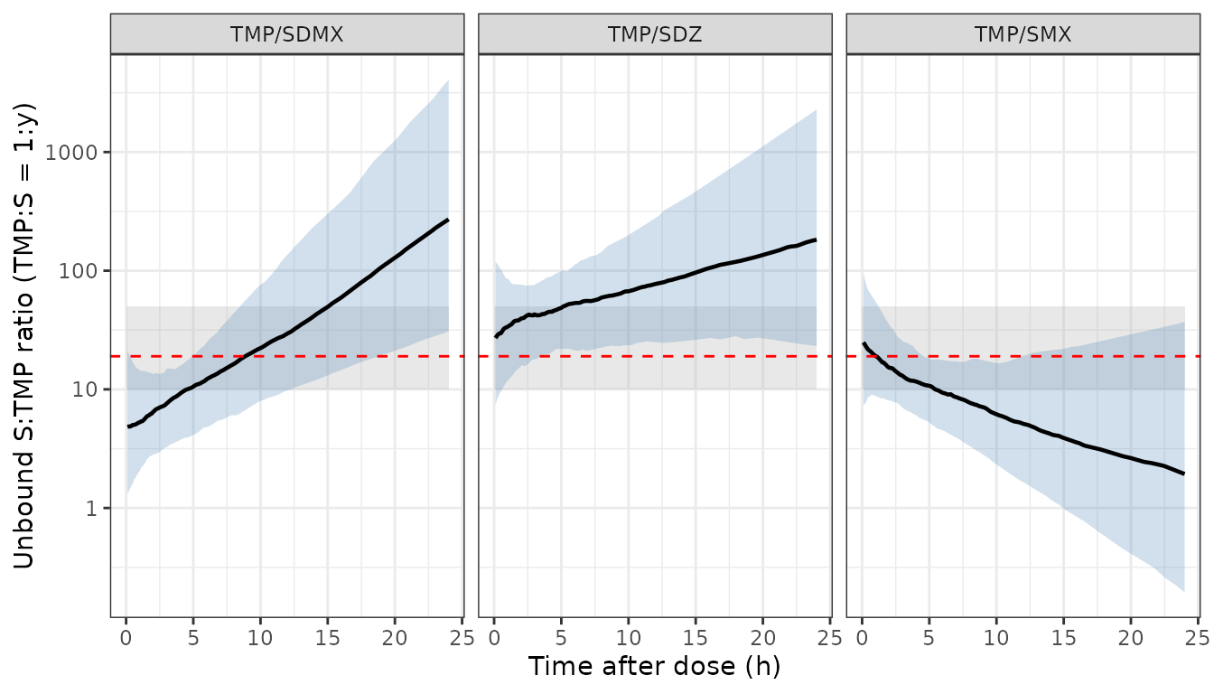

Median (line) and 5th-95th percentile (band) of the unbound sulfonamide:TMP concentration ratio over 24 h after a single oral dose at the registered regimen, n = 200 pigs per combination. The dashed red line is the 1:19 target; the grey band is the relaxed 1:10-1:50 window. Replicates Figure 4 of Boulanger 2025.

The three shapes match the paper’s description: TMP/SDZ sits nearly flat and close to the target because SDZ and TMP have similar half-lives (3.7 vs 2.9 h); TMP/SMX climbs steeply because SMX is cleared faster than TMP; TMP/SDMX sits high and rises because SDMX has a 14.8 h half-life against TMP’s 2.9 h.

Duration within the 1:10-1:50 window

The paper reports a median duration inside the window of 4.5 h (18.8% of 24 h) for TMP/SMX, 14 h (58.3%) for TMP/SDZ and 12 h (50%) for TMP/SDMX.

dur <- ratio_sim |>
  dplyr::group_by(combo, id) |>
  dplyr::summarise(hours_in = sum(ratio >= 10 & ratio <= 50) * 0.1, .groups = "drop") |>
  dplyr::group_by(combo) |>
  dplyr::summarise(`Median h in 1:10-1:50` = round(stats::median(hours_in), 1),
                   `% of 24 h` = round(100 * stats::median(hours_in) / 24, 1),
                   .groups = "drop") |>
  dplyr::left_join(
    tibble::tibble(combo = c("TMP/SMX", "TMP/SDZ", "TMP/SDMX"),
                   `Paper median h` = c(4.5, 14, 12),
                   `Paper % of 24 h` = c(18.8, 58.3, 50.0)),
    by = "combo"
  )
knitr::kable(dur, caption = "Median duration of the unbound TMP:S ratio inside the 1:10-1:50 window over 24 h, against the values reported in the Results and Discussion of Boulanger 2025.")

Median duration of the unbound TMP:S ratio inside the 1:10-1:50 window over 24 h, against the values reported in the Results and Discussion of Boulanger 2025.
combo	Median h in 1:10-1:50	% of 24 h	Paper median h	Paper % of 24 h
TMP/SDMX	9.5	39.6	12.0	50.0
TMP/SDZ	5.6	23.3	14.0	58.3
TMP/SMX	5.4	22.7	4.5	18.8

prop_tbl <- ratio_sim |>
  dplyr::group_by(combo, id) |>
  dplyr::summarise(all_24h = all(ratio >= 10 & ratio <= 50),
                   any_24h = any(ratio >= 10 & ratio <= 50), .groups = "drop") |>
  dplyr::group_by(combo) |>
  dplyr::summarise(`% pigs inside for the whole 24 h` = round(100 * mean(all_24h), 1),
                   `% pigs inside at any time` = round(100 * mean(any_24h), 1),
                   .groups = "drop") |>
  dplyr::left_join(
    tibble::tibble(combo = c("TMP/SMX", "TMP/SDZ", "TMP/SDMX"),
                   `Paper % of pigs` = c(8.8, 46.8, 76.5)),
    by = "combo"
  )
knitr::kable(prop_tbl, caption = "Proportion of simulated pigs inside the 1:10-1:50 window, under two readings of the paper's wording.")

Proportion of simulated pigs inside the 1:10-1:50 window, under two readings of the paper’s wording.
combo	% pigs inside for the whole 24 h	% pigs inside at any time	Paper % of pigs
TMP/SDMX	1.0	99.5	76.5
TMP/SDZ	6.5	89.0	46.8
TMP/SMX	11.0	94.5	8.8

These proportions do not reproduce the paper’s, and neither reading recovers its ordering: under the strict reading TMP/SMX matches well (11.0% simulated against 8.8% published) but TMP/SDZ and TMP/SDMX come out far too low, while under the permissive reading all three are far too high. Only the qualitative conclusion survives – the 1:19 target is met transiently at best. The median-duration table above is the better-posed comparison, and it matches for TMP/SMX (5.4 h vs 4.5 h) and TMP/SDMX (9.5 h vs 12 h) while falling short for TMP/SDZ (5.6 h vs 14 h).

Why the duration metric is fragile, and a check that is not

Time-in-window is a threshold-crossing statistic, so it is acutely sensitive to where the ratio sits relative to the window edges. The time-averaged ratio is not, and it follows in closed form from quantities already in the model: AUC_free,S / AUC_free,TMP = (fu_S F_S D_S / CL_S) / (fu_TMP F_TMP D_TMP / CL_TMP). This is computed per pig, using each animal’s own simulated clearances, so it carries the model’s IOV and its cross-drug correlations.

fmap <- c(TMP = 0.58, SDZ = 0.93, SDMX = 0.68, SMX = 0.64)  # Table 2, oral F

auc_ratio <- ratio_sim |>
  dplyr::distinct(combo, sulfa, id, cl, cl_sdz, cl_sdmx, cl_smx) |>
  dplyr::left_join(dplyr::select(spc, combo, amt_tmp, amt_s), by = "combo") |>
  dplyr::mutate(
    CL_s   = dplyr::case_when(sulfa == "SDZ"  ~ cl_sdz,
                              sulfa == "SDMX" ~ cl_sdmx,
                              sulfa == "SMX"  ~ cl_smx),
    auc_s  = fmap[sulfa] * amt_s   / CL_s * fu[sulfa],
    auc_t  = fmap[["TMP"]] * amt_tmp / cl * fu[["TMP"]],
    ratio  = auc_s / auc_t
  ) |>
  dplyr::group_by(combo) |>
  dplyr::summarise(
    `Median free AUC S:TMP` = round(stats::median(ratio), 1),
    `5th pct`  = round(stats::quantile(ratio, 0.05), 1),
    `95th pct` = round(stats::quantile(ratio, 0.95), 1),
    `Inside 10-50` = paste0(round(100 * mean(ratio >= 10 & ratio <= 50), 1), "%"),
    .groups = "drop"
  ) |>
  dplyr::arrange(abs(`Median free AUC S:TMP` - 19))
knitr::kable(auc_ratio, caption = "Per-pig time-averaged unbound S:TMP exposure ratio at the registered oral regimen, ordered by distance from the 1:19 target.")

Per-pig time-averaged unbound S:TMP exposure ratio at the registered oral regimen, ordered by distance from the 1:19 target.
combo	Median free AUC S:TMP	5th pct	95th pct	Inside 10-50
TMP/SDMX	23.1	10.3	43.9	92.5%
TMP/SMX	11.6	5.9	20.6	65%
TMP/SDZ	50.9	21.7	100.1	48.5%

This is a different statistic from the paper’s, so it is offered as a stability check and an explanation, not as a second attempt at the same number. Two things it shows:

TMP/SDMX sits closest to the 1:19 target (median 23.1) and has the highest share inside the window, agreeing with the paper’s qualitative finding that TMP/SDMX achieves the best attainment of the three.
TMP/SDZ sits at roughly 51, hard against the upper edge of the window. That is precisely why its instantaneous time-in-window is the comparison that disagrees: a combination whose average exposure ratio lands on a boundary spends much of each profile on the far side of it, so a threshold-crossing duration becomes very sensitive to small shifts while the average barely moves.

The agreement is not uniform, and the disagreement is worth naming: TMP/SMX lands at 65% inside on this metric, whereas the paper reports it as the worst of the three (8.8%). That is not a contradiction of the paper – SMX has the shortest half-life of the four drugs, so its S:TMP ratio falls steadily and crosses below 10 partway through the interval even though its 24 h average stays just inside. It does mean the time-averaged view flatters TMP/SMX, and the instantaneous duration (5.4 h simulated vs 4.5 h published, the closest of the three) is the metric that captures the paper’s point for that combination. No parameter was adjusted to move any of these numbers.

Assumptions and deviations

Equations 2 and 3 were transcribed from the article, not assumed. Both display equations are lost by the markdown conversion of the PDF (they render as formula-not-decoded), but they extract cleanly from the PDF’s layout text and are quoted verbatim above. No reconstruction was needed. The four worked covariate examples in the Discussion are retained as an independent check and reproduce to the paper’s stated precision.
Number of occasions. The paper reports one IOV standard deviation per parameter but does not state how many occasions the estimation used. Table 1 describes two cross-over periods plus a third intramuscular period for eight TMP/SDZ pigs, so the model provides three occasion slots (OCC 1-3) sharing a single IOV magnitude – occasions 2 and 3 are fixed() to the occasion-1 value, the equivalent of NONMEM’s $OMEGA BLOCK SAME. Because the magnitude is identical across occasions, this choice does not affect any single-course simulation; it only matters if a user simulates the same animal across periods.
Bioavailability distribution. The paper estimated F on a logit-normal scale to bound it in (0, 1). No inter-individual variability was reported on any F, so the transform has no simulation consequence, and F is encoded on the canonical log scale (lfdepot) as a typical value.
Table S6 typographical correction. One row of Supplementary Table S6 is printed as V2_SDZ - V_SDMX. It is read here as V2_SDZ - V1_SDMX: that is the only pair missing from an otherwise complete set, and with it the table contains exactly 21 entries, the number of off-diagonal pairs of a 7x7 matrix. The resulting covariance matrix is positive definite (eigenvalues 0.734, 0.226, 0.150, 0.069, 0.040, 0.022, 0.0124), so no adjustment was needed to make it simulate.
Random effects not in the correlation block. gamma_Cl_SDMX, gamma_V1_SDZ, gamma_V1_SMX, gamma_V2_SMX and the three omega_ka terms appear in Table 2 but not in Table S6. They are treated as independent, which is the only reading available; the paper does not say whether they were estimated as diagonal or simply omitted from the reported table.
Parameters fixed to zero. IIV and IOV on Q were fixed to zero for all four drugs, as was IIV on ka_SMX (Results, “Population PK analysis”). No random effect is attached to those parameters here, and none is invented. SMX also has no random effect on CL anywhere in Table 2, which is why its simulated AUC has no spread.
The proportion-inside-the-window figures are not reproduced. This is the one published result the extraction does not recover, and it is stated plainly rather than explained away. The paper gives both a proportion of pigs (8.8% / 46.8% / 76.5%) and a median duration (4.5 h / 14 h / 12 h) for the same 1:10-1:50 window, and the two are not mutually consistent under any single reading: a 12 h median duration cannot coexist with 76.5% of pigs “remaining within this interval over 24 h”. Both readings are tabulated above; neither recovers the published ordering. The paper does not state the covariate distribution of its 50,000-pig cohort or the exact definition summarised, so the gap is not attributable from the text alone. No parameter was adjusted to move any of these numbers. Two better-posed checks are reported alongside – median duration, and the closed-form time-averaged exposure ratio – and each agrees with the paper for two of the three combinations, but on different combinations: duration matches TMP/SMX and TMP/SDMX, the exposure ratio matches TMP/SDZ and TMP/SDMX.
TMP/SDZ time-in-window is short (5.6 h simulated vs 14 h published). This has a traceable structural cause rather than being free-floating: at the registered 5 + 25 mg/kg regimen the model’s time-averaged unbound S:TMP ratio for TMP/SDZ is about 51, at the upper edge of the 1:10-1:50 window, so a large share of each profile sits above 50. That in turn follows from the SDZ oral AUC, which is the same starred row in the NCA comparison above: the structural value F x Dose / CL = 0.93 x 25 / 0.12 = 194 exceeds the paper’s pooled Table 3 mean of 144.3, because that mean mixes in De Smet 2017 animals dosed at 12.5 mg/kg. The published mean is therefore not a like-for-like target for a pure 25 mg/kg simulation, and the paper’s own reported range (87.2-220.6) brackets the simulated value.
NCA window truncated at the published LOQ. The TMP/SDMX arms are followed to 168 h so that sulfadimethoxine reaches a quantifiable terminal phase, but trimethoprim underflows to zero long before that, which makes lambda_z – and therefore half.life and aucinf.obs – unestimable for TMP in those arms. Each analyte’s NCA input is therefore truncated at the LOQ reported in the Figure 1 caption (TMP 0.01, SDZ and SDMX 0.1, SMX 0.02 ug/mL), which is the same censoring the real assay applied. This is a property of the simulation grid, not of the model: with the truncation in place the AUCinf = F x Dose / CL identity above holds for every one of the 1400 subject-analyte-route records, TMP included.
De Smet 2017 data. Raw individual SDZ/TMP data from De Smet et al. (2017) were pooled into the original fit. Those data are not reproduced here; the virtual cohort follows the Boulanger 2025 design in Table 1 only. This affects how closely a pooled mean can match Table 3 but not the parameter values.
Analytical exclusions. SMX concentrations after 12 h were discarded by the authors as implausible, so the SMX sub-model is informed only by the first 12 h of data. Simulated SMX profiles beyond 12 h are extrapolations of a two- compartment structure that was never observed over that range.
Cohort sizes. 100 pigs per arm for the NCA comparison and 200 per combination for the ratio simulation, against the paper’s 50,000. This is a deliberate cap for vignette render time; it widens the Monte Carlo error on the percentages in the proportion table but does not change any conclusion.

Session

sessionInfo()
#> R version 4.6.1 (2026-06-24)
#> Platform: x86_64-pc-linux-gnu
#> Running under: Ubuntu 24.04.4 LTS
#> 
#> Matrix products: default
#> BLAS:   /usr/lib/x86_64-linux-gnu/openblas-pthread/libblas.so.3 
#> LAPACK: /usr/lib/x86_64-linux-gnu/openblas-pthread/libopenblasp-r0.3.26.so;  LAPACK version 3.12.0
#> 
#> locale:
#>  [1] LC_CTYPE=C.UTF-8       LC_NUMERIC=C           LC_TIME=C.UTF-8       
#>  [4] LC_COLLATE=C.UTF-8     LC_MONETARY=C.UTF-8    LC_MESSAGES=C.UTF-8   
#>  [7] LC_PAPER=C.UTF-8       LC_NAME=C              LC_ADDRESS=C          
#> [10] LC_TELEPHONE=C         LC_MEASUREMENT=C.UTF-8 LC_IDENTIFICATION=C   
#> 
#> time zone: UTC
#> tzcode source: system (glibc)
#> 
#> attached base packages:
#> [1] stats     graphics  grDevices utils     datasets  methods   base     
#> 
#> other attached packages:
#> [1] ggplot2_4.0.3         tidyr_1.3.2           dplyr_1.2.1          
#> [4] rxode2_5.1.6          PKNCA_0.12.1          nlmixr2lib_0.3.2.9000
#> 
#> loaded via a namespace (and not attached):
#>  [1] gtable_0.3.6        xfun_0.60           bslib_0.12.0       
#>  [4] lattice_0.22-9      vctrs_0.7.3         tools_4.6.1        
#>  [7] generics_0.1.4      parallel_4.6.1      tibble_3.3.1       
#> [10] symengine_0.2.13    pkgconfig_2.0.3     data.table_1.18.6.1
#> [13] checkmate_2.3.4     RColorBrewer_1.1-3  S7_0.2.2           
#> [16] desc_1.4.3          RcppParallel_6.2.1  lifecycle_1.0.5    
#> [19] compiler_4.6.1      farver_2.1.2        textshaping_1.0.5  
#> [22] fontawesome_0.5.3   htmltools_0.5.9     sys_3.4.3          
#> [25] sass_0.4.10         yaml_2.3.12         pillar_1.11.1      
#> [28] pkgdown_2.2.1       crayon_1.5.3        jquerylib_0.1.4    
#> [31] whisker_0.4.1       openssl_2.4.2       cachem_1.1.0       
#> [34] nlme_3.1-169        tidyselect_1.2.1    digest_0.6.39      
#> [37] lotri_1.0.4         purrr_1.2.2         labeling_0.4.3     
#> [40] rxode2ll_2.0.16     fastmap_1.2.0       grid_4.6.1         
#> [43] cli_3.6.6           dparser_1.3.1-13    magrittr_2.0.5     
#> [46] utf8_1.2.6          withr_3.0.3         scales_1.4.0       
#> [49] backports_1.5.1     rmarkdown_2.31      otel_0.2.0         
#> [52] askpass_1.2.1       ragg_1.5.2          memoise_2.0.1      
#> [55] evaluate_1.0.5      knitr_1.51          rex_1.2.2          
#> [58] PreciseSums_0.7     rlang_1.3.0         downlit_0.4.5      
#> [61] Rcpp_1.1.2          glue_1.8.1          xml2_1.6.0         
#> [64] jsonlite_2.0.0      R6_2.6.1            systemfonts_1.3.2  
#> [67] fs_2.1.0