Model and source
- Citation: Ozbey AC, Combarel D, Poinsignon V, Lovera C, Saada E, Mir O, Paci A. Population Pharmacokinetic Analysis of Pazopanib in Patients and Determination of Target AUC. Pharmaceuticals (Basel). 2021;14(9):927. doi:10.3390/ph14090927.
- Description: One-compartment population PK model for oral pazopanib in adult and paediatric cancer patients (therapeutic-drug-monitoring cohort with soft-tissue or Ewing sarcoma, pooled with a phase I/II pazopanib + temozolomide glioblastoma trial), parameterised on apparent clearance and volume with first-order absorption and linear elimination. Aspartate aminotransferase enters V/F as a power model centred at the cohort median of 36.5 U/L. Exponential inter-individual variability on ka, V/F and CL/F, inter-occasion variability on V/F and CL/F, and a combined additive-plus-proportional residual error. Developed to estimate an individual AUC from a single randomly timed sample and to define a target AUC of 750 mg*h/L equivalent to the 20.5 mg/L trough target.
- Article: https://doi.org/10.3390/ph14090927 (open access)
Ozbey et al. built a one-compartment population PK model of oral
pazopanib from therapeutic-drug-monitoring (TDM) samples and full
profiles from a phase I/II trial. The aim was to estimate each patient’s
apparent clearance from a single sample taken at any time after the
dose, and then the AUC as AUC = Dose / (CL/F). Comparing
those AUCs with the observed troughs gave a target AUC of 750 mg*h/L,
which matches the established 20.5 mg/L trough target.
Population
The model was fitted to 73 patients (Methods 4.1, Table 4):
- 58 patients from routine pazopanib TDM at Gustave Roussy between
2012 and
- These were 55 adults and 3 children treated for soft-tissue sarcoma or Ewing sarcoma, contributing 126 samples (1-6 per patient, drawn at a mean of 24.6 h post-dose).
- 15 adults with glioblastoma from a phase I/II trial of pazopanib plus temozolomide (NCT02331498). They had full 0-24 h profiles (0, 0.5, 1, 2, 4, 6, 8 and 24 h) on day 1 of cycles 1, 2 and 4, giving 36 profiles and 280 samples.
Pazopanib was given orally at 200-800 mg once daily; 52 patients were dosed fasted, 15 fed and 6 unknown. In Table 4, age ranges from 3 to 87 years (median 50.5), 44 patients are male and 29 female, and aspartate aminotransferase (ASAT) has a median of 36.5 UI/L (range 22.0-233). Missing covariate values were imputed with the patient’s own median, or failing that the population median. That imputation explains why the ASAT interquartile range (35.4-37.0) is so narrow. Race, body weight and height are not reported.
The same information is available programmatically via
readModelDb("Ozbey_2021_pazopanib")()$population.
Source trace
The per-parameter origin is recorded as an in-file comment next to
each ini() entry in
inst/modeldb/specificDrugs/Ozbey_2021_pazopanib.R. The
table below collects them in one place for review.
| Equation / parameter | Value | Source location |
|---|---|---|
| One-compartment, first-order absorption, linear elimination | n/a | Results paragraph 1; Methods 4.3 |
lka (ka) |
log(0.976) 1/h | Table 1 row ka, RSE 12.3% |
lvc (V/F at ASAT 36.5 UI/L) |
log(22.3) L | Table 1 row V/F, RSE 9.25% |
lcl (CL/F) |
log(0.458) L/h | Table 1 row Cl/F, RSE 9.73% |
e_ast_vc |
-0.838 | Table 1 covariate column; Methods Equation 4 |
| ASAT centring value | 36.5 UI/L | Methods text below Equation 4; Table 4 median |
etalka |
0.211^2 = 0.044521 | Table 1 IIV column (SD scale, see below) |
etalvc |
0.248^2 = 0.061504 | Table 1 IIV column (SD scale) |
etalcl |
0.714^2 = 0.509796 | Table 1 IIV column (SD scale) |
etaiov_vc_1..6 |
0.384^2 = 0.147456 | Table 1 IOV column (SD scale); Methods Equation 1 |
etaiov_cl_1..6 |
0.371^2 = 0.137641 | Table 1 IOV column (SD scale); Methods Equation 2 |
addSd |
4.9 mg/L | Table 1 row Constant residual error, RSE 8.07% |
propSd |
0.05 | Table 1 row Proportional residual error, RSE 26.2% |
vc <- exp(lvc + etalvc + iov_vc) * (AST / 36.5)^e_ast_vc |
n/a | Methods Equations 1 and 4 |
cl <- exp(lcl + etalcl + iov_cl) |
n/a | Methods Equation 2 |
Cc ~ add(addSd) + prop(propSd) + combined1() |
n/a | Methods 4.3 (‘combined model’); Monolix 2018 combined1 form |
Scale of the variability terms
The Table 1 footnote says that “inter-individual variability (IIV) is expressed in omega^2”. The printed values are nonetheless Monolix standard deviations (omega), for two reasons:
- The Results text reads the V/F entry 0.248 directly as a coefficient of variation: ASAT “helped to decrease the inter-individual variability of V/F from 39.8% to 24.8%”.
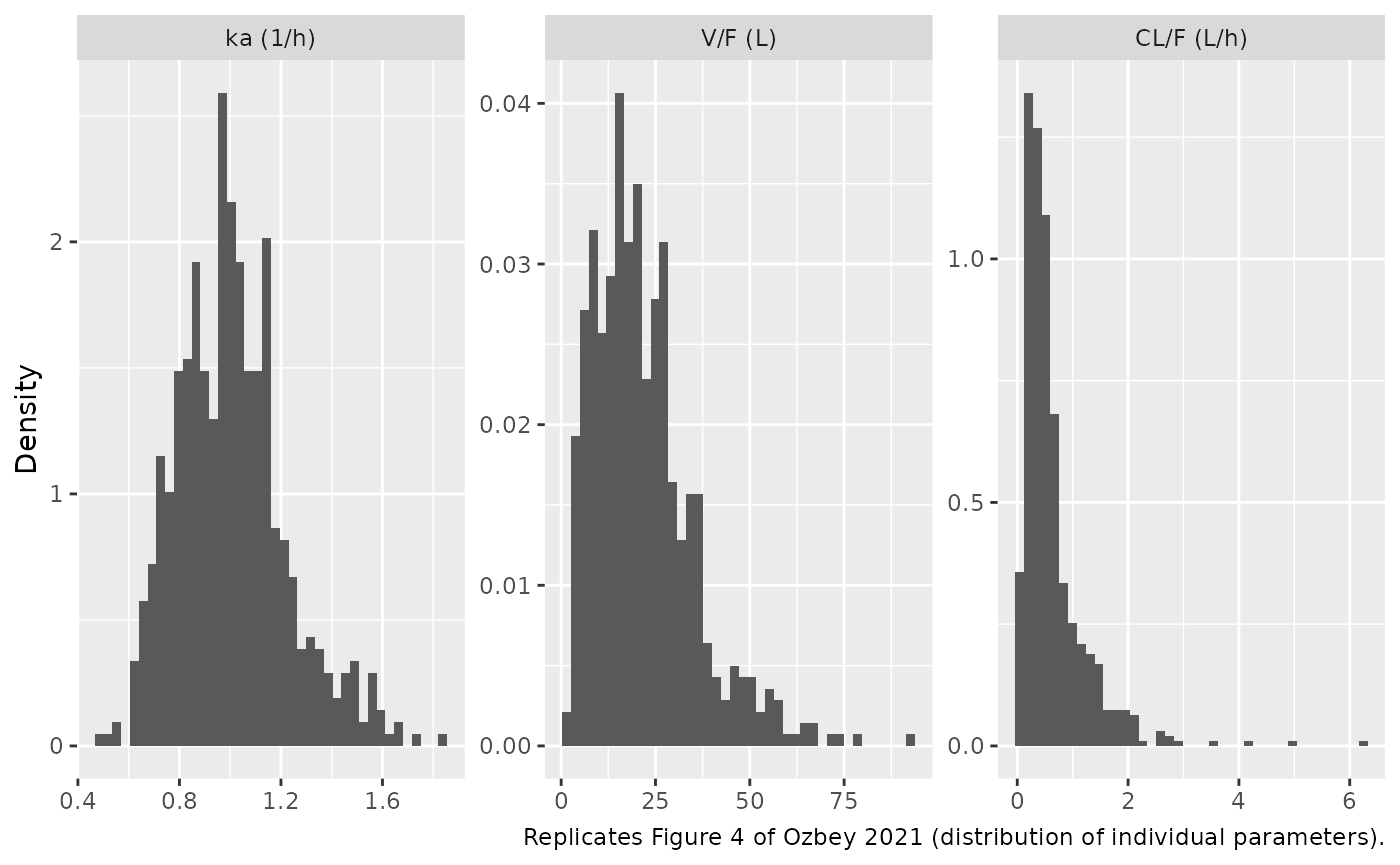
- Figure 4 plots the population distribution of each individual
parameter. For a log-normal with median
mand log-scale SDs, the mode ism * exp(-s^2)and the density at the mode isexp(s^2 / 2) / (m * s * sqrt(2 * pi)).
The ka panel is the cleanest test, because ka carries neither IOV nor a covariate. The curve peaks at a density of about 2 near ka = 0.9 per hour. The V/F and CL/F panels include the IOV term, which Monolix adds to the occasion-level parameter. Their curves have modes near 18 L and 0.2-0.25 L/h. All three were read off Figure 4 by the maintainers.
m <- c(ka = 0.976, vc = 22.3, cl = 0.458)
iiv <- c(ka = 0.211, vc = 0.248, cl = 0.714)
iov <- c(ka = 0, vc = 0.384, cl = 0.371)

lnorm_mode <- function(m, s) m * exp(-s^2)
lnorm_peak <- function(m, s) exp(s^2 / 2) / (m * s * sqrt(2 * pi))

s_sd <- sqrt(iiv^2 + iov^2)   # table values read as SDs
s_var <- sqrt(iiv + iov)      # table values read as variances

omega_check <- tibble(
  parameter = c("ka (1/h)", "V/F (L)", "CL/F (L/h)"),
  figure4_mode = c("~0.9", "~18", "0.20-0.25"),
  mode_sd_reading = signif(lnorm_mode(m, s_sd), 3),
  mode_variance_reading = signif(lnorm_mode(m, s_var), 3),
  peak_sd_reading = signif(lnorm_peak(m, s_sd), 3),
  peak_variance_reading = signif(lnorm_peak(m, s_var), 3)
)

omega_check |>
  dplyr::rename(
    "Parameter" = parameter,
    "Figure 4 mode (digitised)" = figure4_mode,
    "Mode, SD reading" = mode_sd_reading,
    "Mode, variance reading" = mode_variance_reading,
    "Peak density, SD reading" = peak_sd_reading,
    "Peak density, variance reading" = peak_variance_reading
  ) |>
knitr::kable(caption = "Figure 4 parameter distributions under the two readings of Table 1.")| Parameter | Figure 4 mode (digitised) | Mode, SD reading | Mode, variance reading | Peak density, SD reading | Peak density, variance reading |
|---|---|---|---|---|---|
| ka (1/h) | ~0.9 | 0.934 | 0.790 | 1.9800 | 0.9890 |
| V/F (L) | ~18 | 18.100 | 11.900 | 0.0434 | 0.0309 |
| CL/F (L/h) | 0.20-0.25 | 0.240 | 0.155 | 1.5000 | 1.4400 |
# Deterministic arithmetic. The ka curve in Figure 4 peaks at a density of
# about 2 (tallest histogram bars 2.2-2.3). The SD reading gives 1.98 and the
# variance reading 0.99, so it discriminates by a factor of 2. The
# V/F mode (Figure 4: about 18 L) separates the readings the same way:
# 18.1 L versus 11.9 L.
stopifnot(
  abs(lnorm_peak(m[["ka"]], s_sd[["ka"]]) - 2) < 0.3,
  abs(lnorm_peak(m[["ka"]], s_var[["ka"]]) - 2) > 0.8,
  abs(lnorm_mode(m[["vc"]], s_sd[["vc"]]) - 18) < 2,
  abs(lnorm_mode(m[["vc"]], s_var[["vc"]]) - 18) > 5
)
Only the SD reading reproduces Figure 4, so the packaged model uses the squared Table 1 values as the variances.
Virtual cohort
Individual data are not public. The virtual cohort has 150 subjects
in each of four once-daily dose groups spanning the paper’s 200-800 mg
range. ASAT is drawn by interpolating the empirical quantile function
through the Table 4 minimum, quartiles and maximum, so the virtual ASAT
distribution reproduces Table 4. Every subject is simulated at steady
state on a single occasion (OCC = 1).
# rxode2's simulation RNG is partitioned per solver thread, so this cohort is
# reproducible on a given machine but not across thread counts. Every
# assertion on the cohort below is written to hold for any draw the model can
# produce.
rxode2::rxSetSeed(20210915)
set.seed(20210915)

ast_q <- c(22.0, 35.4, 36.5, 37.0, 233) # Table 4: min, Q1, median, Q3, max
draw_ast <- function(n) stats::approx(c(0, 0.25, 0.5, 0.75, 1), ast_q, xout = stats::runif(n))$y

obs_times <- c(0, 0.5, 1, 2, 3, 4, 6, 8, 12, 16, 20, 24)

make_cohort <- function(n, dose, id_offset = 0L) {
  subj <- tibble(
    id = id_offset + seq_len(n),
    AST = draw_ast(n),
    OCC = 1L,
    treatment = paste(dose, "mg QD")
  )
  dosing <- subj |>
    mutate(time = 0, evid = 1L, amt = dose, ii = 24, ss = 1L, cmt = "depot")
  obs <- subj |>
    tidyr::crossing(time = obs_times) |>
    mutate(evid = 0L, amt = 0, ii = 0, ss = 0L, cmt = "central")
  bind_rows(dosing, obs) |>
    arrange(id, time, desc(evid))
}

doses <- c(200, 400, 600, 800)
events <- bind_rows(lapply(seq_along(doses), function(i) {
  make_cohort(150L, doses[i], id_offset = (i - 1L) * 150L)
}))
stopifnot(!anyDuplicated(unique(events[, c("id", "time", "evid")])))
Simulation
mod <- readModelDb("Ozbey_2021_pazopanib")

sim <- rxode2::rxSolve(
  mod,
  events = events,
  keep = c("treatment", "AST"),
  maxsteps = 1e6
) |>
  as.data.frame()
#> Warning: some etas defaulted to non-mu referenced, possible parsing error: etaiov_vc_1, etaiov_vc_2, etaiov_vc_3, etaiov_vc_4, etaiov_vc_5, etaiov_vc_6, etaiov_cl_1, etaiov_cl_2, etaiov_cl_3, etaiov_cl_4, etaiov_cl_5, etaiov_cl_6
#> as a work-around try putting the mu-referenced expression on a simple line

mod_typical <- mod |> rxode2::zeroRe()
#> Warning: some etas defaulted to non-mu referenced, possible parsing error: etaiov_vc_1, etaiov_vc_2, etaiov_vc_3, etaiov_vc_4, etaiov_vc_5, etaiov_vc_6, etaiov_cl_1, etaiov_cl_2, etaiov_cl_3, etaiov_cl_4, etaiov_cl_5, etaiov_cl_6
#> as a work-around try putting the mu-referenced expression on a simple line
#> Warning: some etas defaulted to non-mu referenced, possible parsing error: etaiov_vc_1, etaiov_vc_2, etaiov_vc_3, etaiov_vc_4, etaiov_vc_5, etaiov_vc_6, etaiov_cl_1, etaiov_cl_2, etaiov_cl_3, etaiov_cl_4, etaiov_cl_5, etaiov_cl_6
#> as a work-around try putting the mu-referenced expression on a simple line
events_typical <- events |>
  filter(id %in% c(1L, 151L, 301L, 451L)) |>
  mutate(AST = 36.5)
sim_typical <- rxode2::rxSolve(
  mod_typical,
  events = events_typical,
  keep = c("treatment"),
  maxsteps = 1e6,
  rtol = 1e-10,
  atol = 1e-12,
  ssRtol = 1e-10,
  ssAtol = 1e-12
) |>
  as.data.frame()
#> ℹ omega/sigma items treated as zero: 'etalka', 'etalvc', 'etalcl', 'etaiov_vc_1', 'etaiov_vc_2', 'etaiov_vc_3', 'etaiov_vc_4', 'etaiov_vc_5', 'etaiov_vc_6', 'etaiov_cl_1', 'etaiov_cl_2', 'etaiov_cl_3', 'etaiov_cl_4', 'etaiov_cl_5', 'etaiov_cl_6'
#> Warning: multi-subject simulation without without 'omega'
Typical-value checks
At the median ASAT the typical half-life is
log(2) * V/F / (CL/F). For steady-state once-daily dosing,
the paper computes AUC as Dose / (CL/F).
t_half <- log(2) * 22.3 / 0.458
t_half
#> [1] 33.74931

typ <- sim_typical |>
  group_by(treatment) |>
  summarise(
    ctrough = Cc[time == 24],
    ctrough_t0 = Cc[time == 0],
    cmax = max(Cc),
    .groups = "drop"
  )
knitr::kable(typ, digits = 2, caption = "Typical-value steady-state trough and peak (mg/L), ASAT 36.5 UI/L.")| treatment | ctrough | ctrough_t0 | cmax |
|---|---|---|---|
| 200 mg QD | 14.38 | 14.38 | 21.64 |
| 400 mg QD | 28.76 | 28.76 | 43.29 |
| 600 mg QD | 43.14 | 43.14 | 64.93 |
| 800 mg QD | 57.52 | 57.52 | 86.58 |
# The pre-dose value at t = 0 of an ss = 1 dose is the steady-state trough,
# so it must equal the 24-h value. A mis-set ss record breaks this.
stopifnot(max(abs(typ$ctrough_t0 / typ$ctrough - 1)) < 1e-4)
The typical half-life is 33.7 h. The paper’s Introduction quotes a label half-life of 30.9 h.
Replicate published figures
Figure 2 – visual predictive check
Figure 2 of Ozbey 2021 is a Monolix VPC of concentration against time
after dose (0-30 h), pooling every dose level and occasion. Its observed
median runs from about 35-40 mg/L near the 2-4 h peak to about 20 mg/L
at 24 h. The 90% prediction band spans roughly 5 to 60-100 mg/L. The
simulated band below includes residual error (sim) and
pools the four virtual dose groups.
vpc <- sim |>
  group_by(time) |>
  summarise(
    Q05 = quantile(sim, 0.05, na.rm = TRUE),
    Q50 = quantile(sim, 0.50, na.rm = TRUE),
    Q95 = quantile(sim, 0.95, na.rm = TRUE),
    .groups = "drop"
  )

ggplot(vpc, aes(time, Q50)) +
  geom_ribbon(aes(ymin = Q05, ymax = Q95), alpha = 0.25) +
  geom_line() +
  labs(
    x = "Time after dose (h)",
    y = "Pazopanib concentration (mg/L)",
    title = "Steady-state VPC, 200-800 mg once daily pooled",
    caption = "Replicates Figure 2 of Ozbey 2021 (5th, 50th, 95th percentiles)."
  )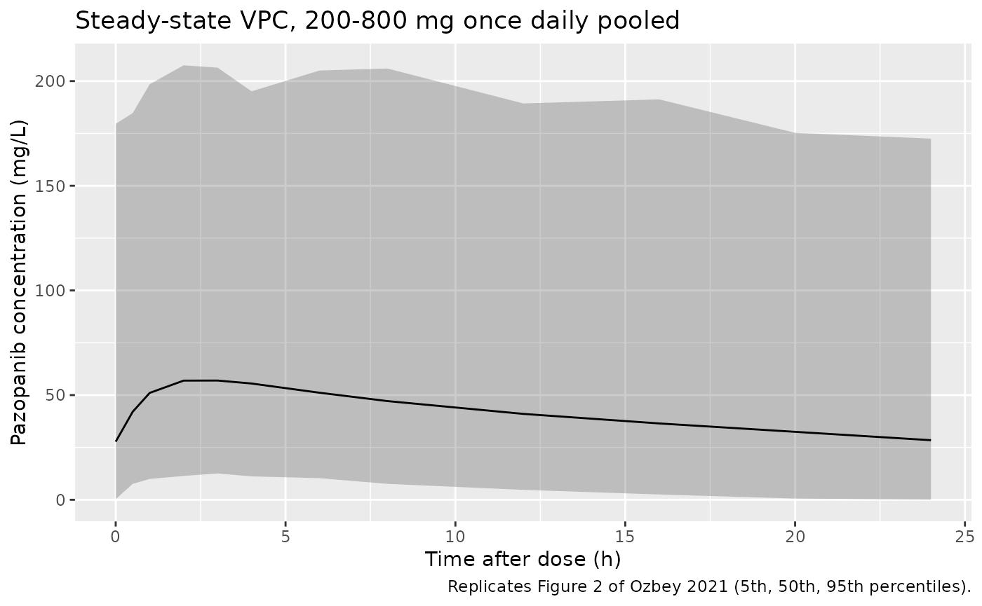
The simulated band has the same shape and order of magnitude as Figure 2. Figure 2 also contains first-dose profiles (cycle 1, day 1) and an unknown mix of dose levels, so a point-by-point comparison is not possible.
Figure 4 – distribution of individual parameters
par_df <- sim |>
  distinct(id, ka, vc, cl) |>
  tidyr::pivot_longer(c(ka, vc, cl), names_to = "parameter", values_to = "value") |>
  mutate(parameter = factor(parameter, c("ka", "vc", "cl"), c("ka (1/h)", "V/F (L)", "CL/F (L/h)")))

ggplot(par_df, aes(value)) +
  geom_histogram(aes(y = after_stat(density)), bins = 40) +
  facet_wrap(~parameter, scales = "free") +
  labs(
    x = NULL, y = "Density",
    caption = "Replicates Figure 4 of Ozbey 2021 (distribution of individual parameters)."
  )
PKNCA validation
The typical-value steady-state profiles are run through PKNCA over
the 0-24 h dosing interval. The reference values are the paper’s own
Dose / (CL/F) AUC formula evaluated at the Table 1
CL/F.
nca_input <- function(d) {
  d |>
    filter(!is.na(Cc)) |>
    select(id, time, Cc, treatment)
}

dose_input <- function(ids) {
  events |>
    filter(evid == 1, id %in% ids) |>
    select(id, time, amt, treatment)
}

intervals <- data.frame(
  start = 0, end = 24,
  cmax = TRUE, tmax = TRUE, cmin = TRUE, auclast = TRUE
)

nca_typ <- PKNCA::pk.nca(PKNCA::PKNCAdata(
  PKNCA::PKNCAconc(nca_input(sim_typical), Cc ~ time | treatment + id),
  PKNCA::PKNCAdose(dose_input(unique(sim_typical$id)), amt ~ time | treatment + id),
  intervals = intervals
))

published <- tibble(
  treatment = paste(doses, "mg QD"),
  auclast = doses / 0.458
)

cmp <- nlmixr2lib::ncaComparisonTable(
  simulated = nca_typ,
  reference = published,
  by = "treatment",
  units = c(auclast = "mg*h/L", cmax = "mg/L", cmin = "mg/L", tmax = "h"),
  tolerance_pct = 20
)
knitr::kable(
  cmp,
  caption = "Typical-value steady-state NCA vs the paper's AUC = Dose / (CL/F). * differs by >20%."
)| NCA parameter | treatment | Reference | Simulated | % diff |
|---|---|---|---|---|
| AUClast (mg*h/L) | 200 mg QD | 437 | 436 | -0.1% |
| AUClast (mg*h/L) | 400 mg QD | 873 | 872 | -0.1% |
| AUClast (mg*h/L) | 600 mg QD | 1310 | 1310 | -0.1% |
| AUClast (mg*h/L) | 800 mg QD | 1750 | 1740 | -0.1% |
auc_typ <- as.data.frame(nca_typ$result) |>
  filter(PPTESTCD == "auclast") |>
  left_join(published, by = "treatment")
# Same drawn (zero) parameters on both sides: the only difference is the
# trapezoidal error of the 12-point grid across the absorption peak.
stopifnot(max(abs(auc_typ$PPORRES / auc_typ$auclast - 1)) < 0.02)
The stochastic cohort goes through the same PKNCA block, split by dose group:
nca_sim <- PKNCA::pk.nca(PKNCA::PKNCAdata(
  PKNCA::PKNCAconc(nca_input(sim), Cc ~ time | treatment + id),
  PKNCA::PKNCAdose(dose_input(unique(sim$id)), amt ~ time | treatment + id),
  intervals = intervals
))

as.data.frame(nca_sim$result) |>
  group_by(treatment, PPTESTCD) |>
  summarise(median = median(PPORRES, na.rm = TRUE), .groups = "drop") |>
  tidyr::pivot_wider(names_from = PPTESTCD, values_from = median) |>
  dplyr::rename(
    "Dose group" = treatment,
    "AUC0-24 (mg*h/L)" = auclast,
    "Cmax (mg/L)" = cmax,
    "Cmin (mg/L)" = cmin,
    "Tmax (h)" = tmax
  ) |>
knitr::kable(digits = 1, caption = "Median steady-state NCA of the virtual cohort.")| Dose group | AUC0-24 (mg*h/L) | Cmax (mg/L) | Cmin (mg/L) | Tmax (h) |
|---|---|---|---|---|
| 200 mg QD | 453.5 | 24.2 | 12.9 | 3 |
| 400 mg QD | 836.4 | 48.7 | 26.1 | 3 |
| 600 mg QD | 1343.5 | 73.2 | 42.0 | 3 |
| 800 mg QD | 1626.1 | 94.8 | 47.3 | 3 |
Target AUC of 750 mg*h/L
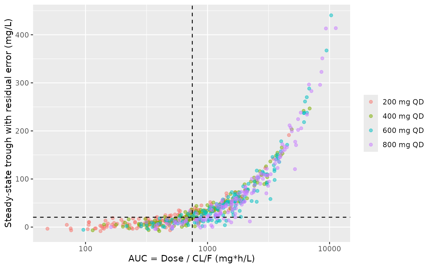
The paper’s central result links the 20.5 mg/L trough target to an AUC target. Among the patients’ model-based AUCs (Dose / individual CL/F), a cut-off of 750 mg*h/L separated troughs above and below 20.5 mg/L with a sensitivity of 99.1% and a specificity of 90.6% (Table 2; the maximum Youden index, 89.8, is at > 743.9 mg*h/L). The trough-AUC correlation coefficient was 0.919.
The same analysis is repeated on the virtual cohort. Each subject’s
AUC is Dose / CL_i, and the trough is the 24-h
concentration including residual error. This is how a TDM trough would
be measured.
per_subj <- sim |>
  filter(time == 24) |>
  transmute(
    id, treatment,
    dose = as.numeric(sub(" mg QD", "", treatment)),
    auc = dose / cl,
    ctrough = sim
  )

roc <- tibble(cutoff = seq(300, 1500, by = 5)) |>
  rowwise() |>
  mutate(
    sensitivity = mean(per_subj$auc[per_subj$ctrough > 20.5] > cutoff),
    specificity = mean(per_subj$auc[per_subj$ctrough <= 20.5] <= cutoff),
    youden = sensitivity + specificity - 1
  ) |>
  ungroup()

best <- roc |> slice_max(youden, n = 1, with_ties = FALSE)
at750 <- roc |> filter(cutoff == 750)
r_ctrough_auc <- cor(per_subj$ctrough, per_subj$auc)

tibble(
  quantity = c("Optimal AUC cut-off (mg*h/L)", "Sensitivity at 750 (%)", "Specificity at 750 (%)", "Pearson r (Ctrough, AUC)"),
  simulated = c(best$cutoff, 100 * at750$sensitivity, 100 * at750$specificity, r_ctrough_auc),
  published = c(743.9, 99.1, 90.6, 0.919)
) |>
  dplyr::rename("Quantity" = quantity, "Simulated" = simulated, "Ozbey 2021" = published) |>
knitr::kable(digits = 3, caption = "Target-AUC analysis: virtual cohort vs Table 2 and Results.")| Quantity | Simulated | Ozbey 2021 |
|---|---|---|
| Optimal AUC cut-off (mg*h/L) | 885.000 | 743.900 |
| Sensitivity at 750 (%) | 90.960 | 99.100 |
| Specificity at 750 (%) | 81.707 | 90.600 |
| Pearson r (Ctrough, AUC) | 0.979 | 0.919 |
ggplot(per_subj, aes(auc, ctrough, colour = treatment)) +
  geom_point(alpha = 0.5) +
  geom_hline(yintercept = 20.5, linetype = 2) +
  geom_vline(xintercept = 750, linetype = 2) +
  scale_x_log10() +
  labs(
    x = "AUC = Dose / CL/F (mg*h/L)",
    y = "Steady-state trough with residual error (mg/L)",
    colour = NULL
  )
# The Youden-optimal cut-off is the argmax of a flat curve, so it is not gated:
# across 13 draws it ranged 705-905 mg*h/L. The gates are instead the
# classification performance AT the published 750 target, which is stable
# across the same draws: sensitivity 0.895-0.944, specificity 0.817-0.906,
# r 0.973-0.987, and a Youden index at most 0.06 below the maximum. A CL/F or
# V/F mis-transcribed by a factor of 2 moves the AUC-trough mapping enough to
# fail one of them.
youden750 <- at750$youden
stopifnot(
  at750$sensitivity > 0.8,
  at750$specificity > 0.7,
  youden750 > best$youden - 0.1,
  r_ctrough_auc > 0.9
)
The virtual cohort supports the paper’s target: an AUC of 750 mg*h/L separates steady-state troughs above and below 20.5 mg/L, and its Youden index (0.727) is within 0.1 of the best achievable cut-off (885 mg*h/L). The Youden curve is flat around its maximum, so the optimal cut-off itself changes by roughly 100 mg*h/L from one virtual cohort to the next. The simulated sensitivity and specificity at 750 mg*h/L sit a few points below the published 99.1% and 90.6%. The main reason is that the simulated troughs carry the model’s residual error (4.9 mg/L + 5%), which blurs the classification near 20.5 mg/L. For reference, at the typical ka and V/F, 750 mg*h/L corresponds to a steady-state trough of 24.7 mg/L. The published threshold came from empirical-Bayes clearances in a cohort whose sampling times, dose levels and occasions the virtual cohort does not reproduce.
Assumptions and deviations
- Scale of IIV and IOV. Table 1 is footnoted as omega^2, but the Results text reads 0.248 as 24.8% and only the SD reading reproduces Figure 4 (see “Scale of the variability terms”). The maintainers therefore treat the printed IIV and IOV values as standard deviations and square them.
-
Residual-error form. The paper says only that a
“combined model” was used, without an equation. The maintainers encoded
Monolix 2018R1’s default combined form,
combined1(residual SD = a + b * f), with a = 4.9 mg/L and b = 0.05. The alternativecombined2form (SD = sqrt(a^2 + b^2 f^2)) would give smaller residual SDs at high concentrations. -
Occasions. The paper reports IOV on V/F and CL/F
but not how occasions were delimited. The trial had three profiled
occasions (cycles 1, 2 and 4), and the TDM patients had 1-6 samples
each. Six occasion slots are encoded, and records outside
OCC1-6 carry no IOV. The simulations here useOCC = 1, so the IOV acts as additional between-subject variability. - ASAT distribution. The virtual ASAT values interpolate the Table 4 quantiles. The narrow interquartile range reflects the paper’s median imputation of missing values, not the true spread of ASAT in the cohort.
- Dose groups and food. The dose mix of the source data is not reported, so four equal dose groups (200, 400, 600 and 800 mg) are simulated. Food status was recorded but not tested as a covariate, and the model has no food effect.
- No body-size covariate. The cohort included three children, aged 3 years and up, but no weight effect was retained. The model should not be extrapolated to children.
-
Errata. No correction notice was found for this
article (Crossref
updated-byrecord checked 2026-09-29).