Mycophenolic acid (Wang 2021)
Source:vignettes/articles/Wang_2021_mycophenolic_acid.Rmd
Wang_2021_mycophenolic_acid.RmdModel and source
- Citation: Wang X, Wu Y, Huang J, Shan S, Mai M, Zhu J, Yang M, Shang D, Wu Z, Lan J, Zhong S, Wu M. (2021). Estimation of Mycophenolic Acid Exposure in Heart Transplant Recipients by Population Pharmacokinetic and Limited Sampling Strategies. Front Pharmacol 12:748609. doi:10.3389/fphar.2021.748609
- Description: Two-compartment population PK model for mycophenolic acid (MPA) after oral mycophenolate mofetil (MMF) dispersible tablets in 91 adult Chinese heart transplant recipients on tacrolimus and corticosteroids (Wang 2021). First-order absorption after a lag time, first-order elimination from the central compartment, and bioavailability fixed at 0.95. Concomitant proton-pump inhibitor use lowers F by a factor of 0.724; eGFR (MDRD, modified for Chinese patients) acts linearly on CL/F around 57 mL/min/1.73 m^2; serum albumin acts as a power function on V2/F around 40 g/L (exponent -7.31). The source fitted doses and concentrations in molar units, so the MMF-to-MPA molecular-weight ratio 320.3/433.5 is carried inside the bioavailability: doses are given as mg of MMF and Cc is MPA in mg/L. IIV is exponential on ka, CL/F, V2/F, Q/F, V3/F, lag time and F; residual error is combined proportional (26.1%) plus additive (0.144 mg/L).
- Article: https://doi.org/10.3389/fphar.2021.748609 (open access; the supplementary material holds the model-building table S1, the limited-sampling tables S2-S3 and the pcVPC in Figure S1)
Wang 2021 fitted mycophenolic acid (MPA) concentrations after oral mycophenolate mofetil (MMF) in adult heart transplant recipients, then used the final model to design limited-sampling strategies for estimating the 12-h AUC. Only the population PK model is packaged here. The paper’s multiple linear regression shortcut (AUC0-12 = 3.539 C0 + 0.288 C0.5 + 1.349 C1 + 6.773 C4.5) is a regression on concentrations, not a PK model; it is used below as a check on the simulated profiles.
Structure
- Two-compartment disposition (central
V2/F, peripheralV3/F, intercompartmental clearanceQ/F) with first-order eliminationCL/F. - First-order absorption
kaafter a lag timeTlag(Table 2). - Bioavailability fixed at
F = 0.95(Methods, citing Bullingham 1996 and Armstrong 2005), with between-subject variability. - Covariates (Table 2 footnote, Equations 2-4):
-
F = 0.95 x 0.724^PPI– proton-pump inhibitor co-medication during the sampling cycle lowers F by 27.6%. -
CL/F = 7.36 x (1 + (eGFR - 57) x 0.00791)– MDRD eGFR modified for Chinese patients, in mL/min/1.73 m^2. -
V2/F = 5.69 x (ALB / 40)^-7.31– serum albumin in g/L.
-
- Exponential IIV on every structural parameter; combined proportional plus additive residual error.
Dose and concentration units
The Methods state that “the units of MMF doses and MPA concentrations
were unified as moles”. The packaged model takes doses in mg of
MMF and returns Cc as MPA in
mg/L. To do that it multiplies the bioavailability by the
molecular-weight ratio MPA/MMF = 320.3/433.5 = 0.739, the same approach
Suzuki_2024_mycophenolic_acid takes. The published
clearances and volumes are the same in molar and mass units, so this
ratio is the only place the choice shows up. Four parts of the paper
support the molar reading:
- The Methods say so directly.
- The y-axis of the Supplementary Figure S1 pcVPC is labelled in mol/L. Its values (median about 0.017 at 0.5 h) only make sense in mmol/L: 0.017 mmol/L is 5.4 mg/L.
- Supplementary Table S1 reports objective function values near -4720 for 507 observations. With the reported residual error, NONMEM’s -2 log likelihood is about +500 when concentrations are in mg/L, but about -5400 when they are in mmol/L. Only the molar dataset can produce an OFV of -4720.
- The individual predicted AUC0-12 values in Figure 5 (median 35.2 mg h/L, range 7.7-113.0, as quoted in the Discussion) agree with this model’s cohort median to within about 15% (checked below). Without the ratio, the cohort median is more than 50% too high.
Table 3 of the paper is the exception. Its steady-state AUC0-12 values match this model to within rounding only when the ratio is left out (500 mg MMF is treated as 500 mg MPA). The maintainers read Table 3 as a simulation that dropped the molar conversion. The Table 3 check below confirms this: every cell differs from the packaged model by exactly the factor 0.739.
Population
91 adult Chinese recipients of a first heart transplant (84 male, 7 female; age 21-74 years, median 50; weight 33.4-95.0 kg, median 60.0) were studied at one centre in Guangzhou (Table 1). They took MMF dispersible tablets 250-750 mg twice daily (median 500 mg), with tacrolimus and methylprednisolone. Sampling began at least 7 days after surgery (post-operative time 7-1067 days, median 37). Median eGFR was 57.2 mL/min/1.73 m^2 (range 6.3-197.1) and median albumin 40.50 g/L (28.56-57.90). About half the patients took a proton-pump inhibitor (49.5%) or a diuretic (50.5%). The data were 508 plasma samples from 105 sampling cycles, measured by EMIT. Fourteen patients had intensive 12-h profiles; the rest were sampled sparsely at 0.5, 1.5, 4 and 9 h.
The same information is available programmatically via
rxode2::rxode(readModelDb("Wang_2021_mycophenolic_acid"))$population.
Source trace
| Equation / parameter | Value | Source location |
|---|---|---|
lka |
log(0.781) 1/h | Table 2, Ka |
lcl |
log(7.36) L/h | Table 2, CL/F |
lvc |
log(5.69) L | Table 2, V2/F |
lq |
log(17.0) L/h | Table 2, Q/F |
lvp |
log(560) L | Table 2, V3/F |
ltlag |
log(0.408) h | Table 2, Tlag |
lfdepot |
fixed(log(0.95)) | Table 2, ‘F 0.95 FIX’; Methods |
e_conmed_ppi_f |
0.724 | Table 2, theta PPI-F; footnote F = TVF x theta^PPI
|
e_crcl_cl |
0.00791 per mL/min/1.73 m^2 | Table 2, theta eGFR-CL; footnote and Equation 4, centred at 57 |
e_alb_vc |
-7.31 | Table 2, theta ALB-V2; footnote and Equation 3, centred at 40 g/L |
etalka |
0.158904 | Table 2, IIV of Ka 41.5%; log(1 + 0.415^2)
|
etalcl |
0.156785 | Table 2, IIV of CL/F 41.2% |
etalvc |
1.499227 | Table 2, IIV of V2/F 186.5% |
etalq |
0.105161 | Table 2, IIV of Q/F 33.3% |
etalvp |
1.524103 | Table 2, IIV of V3/F 189.5% |
etaltlag |
0.017015 | Table 2, IIV of Tlag 13.1% |
etalfdepot |
0.047686 | Table 2, IIV of F 22.1% |
propSd |
0.261 | Table 2, proportional residual error 26.1% |
addSd |
0.144 mg/L | Table 2, additive residual error |
mw_ratio |
320.3/433.5 | Methods (‘unified as moles’); molecular weights of MPA and MMF |
| Two-compartment ODEs with lagged first-order absorption | n/a | Results, ‘Final PPK Model’; Abstract |
IIV form P = Ptv exp(eta)
|
n/a | Equation 1 |
Virtual cohort
The cohort mimics the Table 1 covariate distributions: eGFR log-normal around the median of 57 mL/min/1.73 m^2, albumin normal around 40.5 g/L (both truncated to the observed ranges), and PPI co-medication in 49.5% of participants. Everyone receives the median dose, 500 mg MMF twice daily, at steady state.
# rxSetSeed() makes the cohort reproducible for a given number of solver
# threads, not across machines; every assertion below is written to hold for
# any cohort the model can produce.
rxode2::rxSetSeed(20211119)
set.seed(20211119)

n_sub <- 200
tau <- 12
obs_times <- sort(unique(c(seq(0, tau, by = 0.25), 4.5)))

cov_df <- tibble(
  id = seq_len(n_sub),
  CRCL = pmin(pmax(exp(rnorm(n_sub, log(57), 0.55)), 6.3), 197.1),
  ALB = pmin(pmax(rnorm(n_sub, 40.5, 5), 28.56), 57.9),
  CONMED_PPI = rbinom(n_sub, 1, 0.495),
  treatment = "MMF 500 mg bid"
)

# One steady-state dose (ss = 1) at time 0, then observations over the dosing
# interval on the ODE state `central`; rxode2 returns Cc on those rows.
make_events <- function(cov, dose = 500) {
  doses <- cov |>
    mutate(time = 0, evid = 1L, amt = dose, ii = tau, ss = 1L, cmt = "depot")
  obs <- cov |>
    tidyr::crossing(time = obs_times) |>
    mutate(evid = 0L, amt = 0, ii = 0, ss = 0L, cmt = "central")
  bind_rows(doses, obs) |>
    arrange(id, time, desc(evid))
}

events <- make_events(cov_df)
stopifnot(!anyDuplicated(unique(events[, c("id", "time", "evid")])))
Simulation
mod <- readModelDb("Wang_2021_mycophenolic_acid")

# maxsteps: the steady-state search is charged against one step budget, and a
# subject drawn with a very large V3/F (IIV 189.5%) equilibrates slowly.
sim <- rxode2::rxSolve(
  mod,
  events = events,
  keep = c("treatment", "CONMED_PPI", "CRCL", "ALB"),
  maxsteps = 1e6
) |>
  as.data.frame()
#> ℹ parameter labels from comments will be replaced by 'label()'
stopifnot(!anyNA(sim$Cc))
Steady-state profiles against the pcVPC
Supplementary Figure S1 is a prediction-corrected VPC in mmol/L. The maintainers digitised its shaded 95% confidence band of the simulated median from the vector image and converted it to mg/L (x 320.3 g/mol). A pcVPC rescales each observation to the median population prediction in its time bin, so the band shows the median concentration for the study’s real mix of doses and covariates. It is shown here for orientation only: the cohort above gives everyone 500 mg, while the study used 250-750 mg.
pcvpc_band <- tribble(
  ~time, ~lo_mmol, ~hi_mmol,
  0,     0.0030,   0.0080,
  0.5,   0.0133,   0.0159,
  1,     0.0130,   0.0275,
  1.5,   0.0130,   0.0190,
  2,     0.0098,   0.0187,
  3,     0.0070,   0.0139,
  4,     0.0075,   0.0098,
  6,     0.0044,   0.0104,
  8,     0.0045,   0.0090,
  9,     0.0050,   0.0070,
  12,    0.0031,   0.0083
) |>
  mutate(lo = lo_mmol * 320.3, hi = hi_mmol * 320.3)

sim_summary <- sim |>
  group_by(time) |>
  summarise(
    Q05 = quantile(Cc, 0.05),
    Q50 = median(Cc),
    Q95 = quantile(Cc, 0.95),
    .groups = "drop"
  )

ggplot(sim_summary, aes(time, Q50)) +
  geom_ribbon(aes(ymin = Q05, ymax = Q95), alpha = 0.2) +
  geom_line() +
  geom_errorbar(
    data = pcvpc_band,
    aes(x = time, ymin = lo, ymax = hi),
    inherit.aes = FALSE,
    width = 0.25,
    colour = "firebrick"
  ) +
  scale_x_continuous(breaks = seq(0, 12, by = 2)) +
  labs(
    x = "Time after dose (h)",
    y = "MPA concentration (mg/L)",
    title = "Steady-state MPA, MMF 500 mg bid",
    caption = "Error bars: digitised Supplementary Figure S1 of Wang 2021."
  )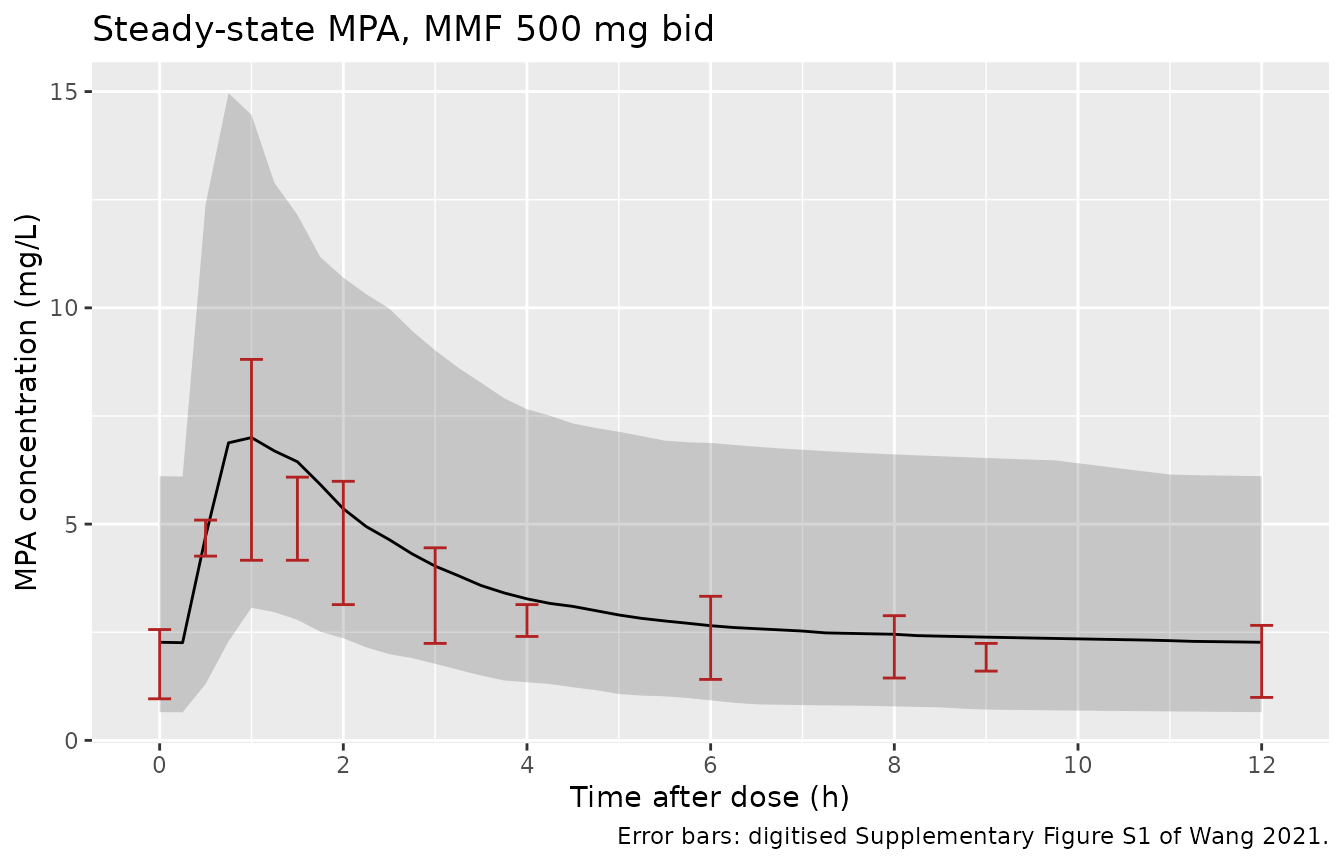
Simulated steady-state MPA concentrations after MMF 500 mg twice daily (200 virtual participants). Line = median, ribbon = 5th-95th percentile of the individual predictions. Error bars = 95% confidence band of the simulated median in Supplementary Figure S1 of Wang 2021, digitised and converted to mg/L.
Replicate Table 3: steady-state AUC0-12 by covariate
Table 3 of the paper gives the typical-value steady-state AUC0-12
after 500 mg MMF twice daily for 24 combinations of PPI use, albumin and
eGFR. The AUC was computed with the linear trapezoidal rule on a 0.5-h
grid of population predictions. The same calculation is repeated here
with PKNCA (auc.method = "linear") on the typical-value
model.
table3 <- tribble(
  ~CONMED_PPI, ~ALB, ~egfr30, ~egfr60, ~egfr90, ~egfr130,
  0, 30, 82.1, 63.0, 51.2, 40.9,
  0, 40, 82.2, 63.2, 51.3, 41.1,
  0, 60, 84.8, 65.5, 53.5, 43.0,
  1, 30, 59.4, 45.6, 37.0, 29.6,
  1, 40, 59.5, 45.7, 37.2, 29.7,
  1, 60, 61.4, 47.4, 38.7, 31.1
) |>
  pivot_longer(starts_with("egfr"), names_to = "CRCL", values_to = "auc_paper") |>
  mutate(CRCL = as.numeric(sub("egfr", "", CRCL)))

scen <- table3 |>
  mutate(
    id = row_number(),
    treatment = sprintf("PPI %d, ALB %g, eGFR %g", CONMED_PPI, ALB, CRCL)
  )

ev_t3 <- scen |>
  select(id, treatment, CONMED_PPI, ALB, CRCL) |>
  tidyr::crossing(time = seq(0, tau, by = 0.5)) |>
  mutate(evid = 0L, amt = 0, ii = 0, ss = 0L, cmt = "central") |>
  bind_rows(
    scen |>
      select(id, treatment, CONMED_PPI, ALB, CRCL) |>
      mutate(time = 0, evid = 1L, amt = 500, ii = tau, ss = 1L, cmt = "depot")
  ) |>
  arrange(id, time, desc(evid))

sim_t3 <- rxode2::rxSolve(
  rxode2::zeroRe(mod),
  events = ev_t3,
  keep = "treatment",
  rtol = 1e-10, atol = 1e-12, ssRtol = 1e-10, ssAtol = 1e-12,
  maxsteps = 1e6
) |>
  as.data.frame()
#> ℹ parameter labels from comments will be replaced by 'label()'
#> ℹ omega/sigma items treated as zero: 'etalka', 'etalcl', 'etalvc', 'etalq', 'etalvp', 'etaltlag', 'etalfdepot'
#> Warning: multi-subject simulation without without 'omega'

t3_conc <- PKNCA::PKNCAconc(
  sim_t3 |> filter(!is.na(Cc)) |> select(id, time, Cc, treatment),
  Cc ~ time | treatment + id
)
t3_dose <- PKNCA::PKNCAdose(
  ev_t3 |> filter(evid == 1) |> select(id, time, amt, treatment),
  amt ~ time | treatment + id
)
t3_nca <- PKNCA::pk.nca(PKNCA::PKNCAdata(
  t3_conc, t3_dose,
  intervals = data.frame(start = 0, end = tau, auclast = TRUE),
  options = list(auc.method = "linear")
))

mw_ratio <- 320.3 / 433.5
t3_cmp <- as.data.frame(t3_nca) |>
  filter(PPTESTCD == "auclast") |>
  select(treatment, auc_model = PPORRES) |>
  inner_join(scen, by = "treatment") |>
  mutate(
    ratio = auc_model / auc_paper,
    auc_model_no_mw = auc_model / mw_ratio
  )
stopifnot(nrow(t3_cmp) == 24L)

t3_cmp |>
  select(CONMED_PPI, ALB, CRCL, auc_paper, auc_model, auc_model_no_mw, ratio) |>
  rename(
    "PPI" = CONMED_PPI,
    "ALB (g/L)" = ALB,
    "eGFR (mL/min/1.73 m^2)" = CRCL,
    "Table 3 AUC0-12 (mg h/L)" = auc_paper,
    "Model AUC0-12 (mg h/L)" = auc_model,
    "Model without MW ratio (mg h/L)" = auc_model_no_mw,
    "Model / Table 3" = ratio
  ) |>
knitr::kable(digits = 3, caption = "Typical-value steady-state AUC0-12 after MMF 500 mg twice daily: Table 3 of Wang 2021 against the packaged model.")| PPI | ALB (g/L) | eGFR (mL/min/1.73 m^2) | Table 3 AUC0-12 (mg h/L) | Model AUC0-12 (mg h/L) | Model without MW ratio (mg h/L) | Model / Table 3 |
|---|---|---|---|---|---|---|
| 0 | 30 | 130 | 40.9 | 30.226 | 40.908 | 0.739 |
| 0 | 30 | 30 | 82.1 | 60.630 | 82.058 | 0.738 |
| 0 | 30 | 60 | 63.0 | 46.575 | 63.036 | 0.739 |
| 0 | 30 | 90 | 51.2 | 37.810 | 51.173 | 0.738 |
| 0 | 40 | 130 | 41.1 | 30.403 | 41.149 | 0.740 |
| 0 | 40 | 30 | 82.2 | 60.766 | 82.242 | 0.739 |
| 0 | 40 | 60 | 63.2 | 46.724 | 63.238 | 0.739 |
| 0 | 40 | 90 | 51.3 | 37.972 | 51.392 | 0.740 |
| 0 | 60 | 130 | 43.0 | 31.863 | 43.124 | 0.741 |
| 0 | 60 | 30 | 84.8 | 62.717 | 84.883 | 0.740 |
| 0 | 60 | 60 | 65.5 | 48.504 | 65.646 | 0.741 |
| 0 | 60 | 90 | 53.5 | 39.602 | 53.599 | 0.740 |
| 1 | 30 | 130 | 29.6 | 21.884 | 29.618 | 0.739 |
| 1 | 30 | 30 | 59.4 | 43.896 | 59.410 | 0.739 |
| 1 | 30 | 60 | 45.6 | 33.721 | 45.638 | 0.739 |
| 1 | 30 | 90 | 37.0 | 27.375 | 37.049 | 0.740 |
| 1 | 40 | 130 | 29.7 | 22.012 | 29.792 | 0.741 |
| 1 | 40 | 30 | 59.5 | 43.995 | 59.544 | 0.739 |
| 1 | 40 | 60 | 45.7 | 33.829 | 45.784 | 0.740 |
| 1 | 40 | 90 | 37.2 | 27.492 | 37.208 | 0.739 |
| 1 | 60 | 130 | 31.1 | 23.069 | 31.222 | 0.742 |
| 1 | 60 | 30 | 61.4 | 45.407 | 61.455 | 0.740 |
| 1 | 60 | 60 | 47.4 | 35.117 | 47.528 | 0.741 |
| 1 | 60 | 90 | 38.7 | 28.672 | 38.805 | 0.741 |
In every cell, the packaged model divided by Table 3 is the molecular-weight ratio 0.7389. If the ratio is left out, the model reproduces Table 3 to within 0.39% in every cell. The model’s structure, including the albumin, eGFR and PPI terms, is therefore transcribed correctly. The only remaining difference is the molar dose conversion, discussed above.
# Deterministic check (typical values, tight solver tolerances). Table 3 is
# printed to 0.1 mg h/L, i.e. <= 0.17% of its smallest entry; the largest
# realised deviation from the MW ratio was 0.39%, slightly above print
# rounding (the paper does not say how it reached steady state). A mis-transcribed
# coefficient moves whole rows or columns by several percent, and dropping or
# doubling the MW ratio moves every cell by 26-35%.
stopifnot(max(abs(t3_cmp$ratio / mw_ratio - 1)) < 0.01)
PKNCA validation
sim_nca <- sim |>
  filter(!is.na(Cc)) |>
  select(id, time, Cc, treatment)

dose_df <- events |>
  filter(evid == 1) |>
  select(id, time, amt, treatment)

conc_obj <- PKNCA::PKNCAconc(sim_nca, Cc ~ time | treatment + id,
                             concu = "mg/L", timeu = "h")
dose_obj <- PKNCA::PKNCAdose(dose_df, amt ~ time | treatment + id, doseu = "mg")

intervals <- data.frame(
  start = 0,
  end = tau,
  cmax = TRUE,
  tmax = TRUE,
  cmin = TRUE,
  auclast = TRUE,
  cav = TRUE
)

nca_res <- PKNCA::pk.nca(PKNCA::PKNCAdata(
  conc_obj, dose_obj,
  intervals = intervals,
  options = list(auc.method = "linear")
))
nca_ind <- as.data.frame(nca_res) |>
  select(id, PPTESTCD, PPORRES) |>
  inner_join(cov_df |> select(id, CONMED_PPI), by = "id")

nca_ind |>
  filter(PPTESTCD %in% c("cmax", "tmax", "cmin", "cav", "auclast")) |>
  mutate(PPI = if_else(CONMED_PPI == 1, "With PPI", "Without PPI")) |>
  group_by(PPI, PPTESTCD) |>
  summarise(median = median(PPORRES), .groups = "drop") |>
  pivot_wider(names_from = PPTESTCD, values_from = median) |>
  select(PPI, cmax, tmax, cmin, cav, auclast) |>
  rename(
    "PPI co-medication" = PPI,
    "Cmax,ss (mg/L)" = cmax,
    "Tmax (h)" = tmax,
    "Cmin,ss (mg/L)" = cmin,
    "Cavg,ss (mg/L)" = cav,
    "AUC0-12 (mg h/L)" = auclast
  ) |>
knitr::kable(digits = 2, caption = "Median steady-state NCA parameters after MMF 500 mg twice daily, by PPI co-medication.")| PPI co-medication | Cmax,ss (mg/L) | Tmax (h) | Cmin,ss (mg/L) | Cavg,ss (mg/L) | AUC0-12 (mg h/L) |
|---|---|---|---|---|---|
| With PPI | 6.86 | 1 | 1.77 | 2.76 | 33.15 |
| Without PPI | 8.46 | 1 | 2.69 | 4.10 | 49.22 |
Comparison against published exposure
The Discussion quotes a median individual predicted AUC0-12 of 35.2 mg h/L (range 7.7-113.0) across the 105 sampling cycles (Figure 5, the AUCipred axis). The cohort-median AUC0-12 from the virtual cohort is compared with it below. The study doses ranged from 250 to 750 mg around the 500 mg median, so this is a comparison of medians, not of the full distribution.
published <- tibble(treatment = "MMF 500 mg bid", auclast = 35.2)

cmp <- nlmixr2lib::ncaComparisonTable(
  simulated = nca_res,
  reference = published,
  by = "treatment",
  params = "auclast",
  units = c(auclast = "mg*h/L"),
  tolerance_pct = 20
)
knitr::kable(cmp, caption = "Simulated vs. published median AUC0-12. * differs from reference by >20%.")| NCA parameter | treatment | Reference | Simulated | % diff |
|---|---|---|---|---|
| AUClast (mg*h/L) | MMF 500 mg bid | 35.2 | 40.7 | +15.5% |
auc_med <- median(nca_ind$PPORRES[nca_ind$PPTESTCD == "auclast"])
auc_range <- range(nca_ind$PPORRES[nca_ind$PPTESTCD == "auclast"])
# Centre, not extremes. With the molar conversion this cohort's median sits
# about 10-16% above 35.2 (40.7 mg h/L realised); the sampling SE of the log
# median of 200 subjects is about 5%, so the 35% bound is >3 SE away. Without
# the conversion the median would be about 55 mg h/L (+56%), which this bound
# rejects.
stopifnot(abs(auc_med / 35.2 - 1) < 0.35)
The simulated median AUC0-12 is 40.7 mg h/L, with a range of 10.2-247.2 mg h/L, against the published median 35.2 (7.7-113.0). Treating the dose as mg of MPA would inflate every value by 1.353-fold.
Limited-sampling equation as a shape check
The paper’s final regression, AUC0-12 = 3.539 C0 + 0.288 C0.5 + 1.349 C1 + 6.773 C4.5 (r^2 = 0.999), was fitted to simulated profiles from this model. It is linear in the concentrations, so it carries no information about the dose scale. It does test the shape of the profiles: if absorption, distribution or lag were transcribed wrongly, it would fail.
mlr <- sim |>
  filter(time %in% c(0, 0.5, 1, 4.5)) |>
  select(id, time, Cc) |>
  pivot_wider(names_from = time, values_from = Cc, names_prefix = "C") |>
  mutate(auc_mlr = 3.539 * C0 + 0.288 * C0.5 + 1.349 * C1 + 6.773 * C4.5) |>
  inner_join(
    nca_ind |> filter(PPTESTCD == "auclast") |> select(id, auc_nca = PPORRES),
    by = "id"
  ) |>
  mutate(pct_diff = 100 * (auc_mlr / auc_nca - 1))

mlr_summary <- tibble(
  "Median % difference" = median(mlr$pct_diff),
  "90th percentile |% difference|" = unname(quantile(abs(mlr$pct_diff), 0.9)),
  "Pearson r" = cor(mlr$auc_mlr, mlr$auc_nca)
)
knitr::kable(mlr_summary, digits = 3, caption = "MLR-estimated vs. PKNCA AUC0-12 in the virtual cohort (the paper reports %ME 0.33% and %RMSE 1.75% against its own AUCipred).")| Median % difference | 90th percentile |% difference| | Pearson r |
|---|---|---|
| 1.01 | 3.458 | 1 |
# Centre and robust envelope. The paper's own agreement was %ME 0.33% and
# %RMSE 1.75%; the virtual cohort's covariate mix differs from the study's, so
# allow some headroom. A wrong ka, tlag or V2 shifts the median by >10%.
stopifnot(
  abs(median(mlr$pct_diff)) < 5,
  quantile(abs(mlr$pct_diff), 0.9) < 15
)
Assumptions and deviations
- Molar dose conversion. The model multiplies F by the MPA/MMF molecular-weight ratio 320.3/433.5. The paper states that doses and concentrations were fitted in moles, but does not print the molecular weights; the standard values used elsewhere in the package are taken. Table 3 of the paper is reproduced exactly only when this ratio is omitted, which the maintainers treat as an error in the paper’s Table 3 simulation (see “Dose and concentration units”).
-
IIV scale. Table 2 prints each IIV as a percentage
without defining it. The maintainers converted it with
omega^2 = log(1 + CV^2). For the small IIVs this is nearly the same as reading the percentage assqrt(omega^2), but not for V2/F (186.5%) and V3/F (189.5%): there the alternative reading gives variances of 3.48 and 3.59 instead of 1.50 and 1.52. The pcVPC spread in Figure S1 is too coarse to tell the two readings apart; they differ by about 10% in the 95th/50th percentile ratio. - No IIV covariances. The Methods mention estimating a variance-covariance matrix, but Table 2 reports no covariances, so the omega matrix is diagonal.
- Additive error units. The additive residual error is reported as 0.144 mg/L and used as-is. In the molar fit NONMEM would have estimated it in mmol/L, so the paper presumably converted it for the table.
-
Covariate definitions.
CONMED_PPIis recorded per PK sampling cycle (omeprazole or pantoprazole, intravenous or oral).CRCLholds the MDRD eGFR modified for Chinese patients (Ma 2006), in mL/min/1.73 m^2.ALBis in g/L. The eGFR term is linear, soCL/Fstays positive for any eGFR above -69 mL/min/1.73 m^2, i.e. for every real value. - Virtual cohort. eGFR is drawn log-normal (median 57, log-SD 0.55) and albumin normal (mean 40.5, SD 5 g/L), both truncated to the Table 1 ranges. PPI use is Bernoulli(0.495). Everyone receives 500 mg twice daily. The paper does not report the dose distribution or covariate correlations.
- pcVPC digitisation. The Figure S1 median band was digitised from the supplementary image’s pixels. At 1.5, 4 and 9 h the band is hidden behind data points and was read by eye. It is plotted for orientation only and is not used in any assertion.
- Enterohepatic recirculation is not in the final model; the authors tried it, and the run did not minimise (Supplementary Table S1, model 3).
- No correction notice for the article was found in Europe PMC as of 2026-09-29.