Ritlecitinib (Purohit 2023)
Source:vignettes/articles/Purohit_2023_ritlecitinib.Rmd
Purohit_2023_ritlecitinib.RmdModel and source
- Citation: Purohit V, Huh Y, Wojciechowski J, Plotka A, Salts S, Antinew J, Dimitrova A, Nicholas T. Leveraging Prior Healthy Participant Pharmacokinetic Data to Evaluate the Impact of Renal and Hepatic Impairment on Ritlecitinib Pharmacokinetics. AAPS J. 2023;25(3):32. doi:10.1208/s12248-023-00792-8. PMCID PMC10047454. Parameter estimates from Supplementary Table B; model equations from the final-model NONMEM control stream (run12.mod) in Supplementary Text S1.
- Description: Two-compartment population pharmacokinetic model with first-order absorption for oral ritlecitinib (PF-06651600, a covalent JAK3/TEC-family kinase inhibitor) in healthy participants and patients with rheumatoid arthritis. Apparent clearance and apparent central volume carry allometric body-weight scaling with exponents fixed at 0.75 and 1 referenced to 75 kg; apparent clearance is lower in rheumatoid arthritis patients and at total daily doses above 100 mg, and a high-fat meal slows absorption. Interindividual variability on CL/F and Vc/F is correlated, and the log-scale residual error differs between healthy participants and rheumatoid arthritis patients. This is the interim (fit-for-purpose) model used to simulate in silico healthy-participant reference cohorts for the ritlecitinib hepatic and renal impairment studies.
- Article: https://doi.org/10.1208/s12248-023-00792-8
Ritlecitinib (PF-06651600) is an oral covalent, irreversible inhibitor of Janus kinase 3 (JAK3) and the TEC kinase family. Purohit 2023 reports the phase I hepatic impairment (moderate, Child-Pugh B; 30 mg QD) and renal impairment (severe, eGFR < 30 mL/min; 50 mg QD) studies. The healthy-participant arm of the renal study was never recruited because of the COVID-19 pause, so the authors generated in silico healthy-participant reference cohorts with an interim population PK model fitted to three earlier studies. That interim model, published in full (NONMEM control stream and parameter table) in Supplementary Text S1, is the model packaged here.
The later models of the same development programme – with an
autoinhibitory Imax effect on clearance and bioavailability, fitted to
far larger alopecia areata datasets – are packaged separately as
Wojciechowski_2023_ritlecitinib_base, _updated
and _final.
Population
The model was fitted to 1519 plasma ritlecitinib concentrations from 113 participants pooled from three studies (Supplementary Text S1 and Table A):
- NCT02309827 – phase I single (5-800 mg) and multiple (50, 200, 400 mg QD; 100, 200 mg BID for 14 days) ascending-dose study in healthy participants, fasted (80 enrolled).
- NCT02684760 – phase I relative-bioavailability and food-effect study in healthy participants: 50 mg tablet fasted, 50 mg oral solution fasted, 50 mg tablet after a high-fat meal (14 enrolled).
- NCT02969044 – phase II study in moderate to severe active rheumatoid arthritis with an inadequate response to methotrexate: 200 mg QD for 8 weeks, fasted, sparse sampling (70 randomized, including placebo).
Baseline demographics of the modelling population are not reported. The two impairment studies that the model was used to support enrolled participants aged 18-75 years weighing more than 50 kg; Table I gives their demographics.
The same information is available programmatically via
readModelDb("Purohit_2023_ritlecitinib")()$population.
Source trace
Every ini() entry in
inst/modeldb/specificDrugs/Purohit_2023_ritlecitinib.R
carries an in-file comment naming its origin. They are collected here
for review.
| Equation / parameter | Value | Source location |
|---|---|---|
lka (ka) |
3.48 1/h (95% CI 3.09-3.87) | Supplementary Table B ‘ka’; control stream THETA(1) |
lcl (CL/F at 75 kg) |
78.1 L/h (70.3-86.0) | Table B ‘CL/F’; THETA(2) |
lvc (Vc/F at 75 kg) |
119 L (99.7-138) | Table B ‘V/F’; THETA(3) |
lq (Q/F) |
0.424 L/h (0.339-0.509) | Table B ‘Q’; THETA(4) |
lvp (Vp/F) |
3.54 L (3.12-3.97) | Table B ‘Vp/F’; THETA(5) |
e_wt_cl |
0.75 (not estimated) | Text S1 ‘Structural Model Development’; control stream
(BWT/75)**0.75
|
e_wt_vc |
1 (not estimated) | Text S1; control stream TVV2 = THETA(3)*(BWT/75)
|
e_dose_high_cl |
log(0.666) | Table B ‘Dose on CL/F’ = 0.666 (0.641-0.691); THETA(7) |
e_dis_ra_cl |
log(0.625) | Table B ‘RA on CL/F’ = 0.625 (0.564-0.739); THETA(10) |
e_fed_highfat_ka |
-0.613 | Table B ‘Food on ka’ = -0.613 (-0.649 to -0.577); THETA(9) |
var(etalcl) |
0.156^2 = 0.024336 | Table B ‘IIV-CL/F’ = 0.156, read as an SD (see below) |
cov(etalcl, etalvc) |
0.173 x 0.156 x 0.280 = 0.00755664 | Table B ‘Cov CL/F-V/F’ = 0.173, read as a correlation |
var(etalvc) |
0.280^2 = 0.0784 | Table B ‘IIV-V/F’ = 0.280, read as an SD |
expSdHv |
sqrt(0.166) = 0.407 | Table B ‘RUV-HP’ (a $SIGMA variance) |
expSdRa |
sqrt(0.860) = 0.927 | Table B ‘RUV-RA’ (a $SIGMA variance) |
| ka | KA = THETA(1)*(1 + FED*THETA(9)) |
control stream $PK (FLG3 = 0 IF (FOOD.NE.0)) |
| CL/F | THETA(2) * THETA(7)^[TDD > 100] * (BWT/75)^0.75 * THETA(10)^RA * exp(ETA(1)) |
control stream $PK (TRT = DOSE*DFREQ) |
| Vc/F | THETA(3) * (BWT/75) * exp(ETA(2)) |
control stream $PK |
| Absorption lag | none (ALAG1 THETAs 6 and 8 are 0 FIX) |
control stream $PK and $THETA |
| Cc (ng/mL) | 1000 * central / vc |
control stream S2 = V2/1000
|
| Residual error |
log(DV) = log(Cc) + eps, SD by population |
control stream $ERROR |
Reading the variability rows of Table B
Table B’s footnote calls the IIV rows ‘inter-individual variance’, and the off-diagonal row is labelled ‘Cov CL/F-V/F’. Taken literally (variances 0.156 and 0.280, covariance 0.173) the block is positive definite, so the label cannot be excluded on arithmetic alone. It does, however, contradict the paper’s own simulation: under that reading the 90% prediction interval of the trial geometric-mean AUC0-24 in Table IV comes out about 2.2-fold too wide, and the implied 45% CV of AUC in healthy participants is far above the 16% observed in the eight Study 1 healthy participants (Table II).
The packaged model therefore reads the IIV rows as NONMEM’s
correlation-matrix print – SDs of 0.156 (CL/F) and 0.280 (Vc/F) on the
diagonal, correlation 0.173 off it – and keeps the residual-error rows
as the labelled $SIGMA variances (0.166 and 0.860, log-scale SDs 0.407
and 0.927). Reading the residual-error rows as SDs as well narrows the
AUC interval further but leaves the simulated Table IV Cmax medians
about 15% short. The section Scale of the variability rows
below repeats the Table IV simulation under all three readings. The
chosen magnitudes are also in line with the later model of the same
programme fitted to overlapping data
(Wojciechowski_2023_ritlecitinib_base: healthy-participant
IIV SD on CL/F 0.201 and on Vc/F 0.113, proportional residual SD
0.340).
Because the control stream fits log-transformed concentrations with
an additive epsilon (Y = LOG(F) + EPS), the log-scale
residual SD for lnorm() is the square root of each $SIGMA
variance.
Deterministic covariate checks
The covariate model is a set of multiplicative switches, so each published coefficient can be verified exactly from typical-value parameters.
mod <- readModelDb("Purohit_2023_ritlecitinib")
mod_typ <- rxode2::zeroRe(mod)
#> ℹ parameter labels from comments will be replaced by 'label()'
#> Warning: No sigma parameters in the model

cov_grid <- tibble::tribble(
  ~scenario,                          ~WT, ~DIS_RA, ~DOSE_HIGH, ~FED_HIGHFAT,
  "Reference (75 kg healthy, fasted)",  75,       0,          0,            0,
  "100 kg healthy",                    100,       0,          0,            0,
  "Rheumatoid arthritis",               75,       1,          0,            0,
  "Total daily dose > 100 mg",          75,       0,          1,            0,
  "High-fat meal",                      75,       0,          0,            1
) |>
  mutate(id = row_number())

ev_cov <- cov_grid |>
  select(id, WT, DIS_RA, DOSE_HIGH, FED_HIGHFAT) |>
  mutate(time = 0, amt = 0, evid = 0, cmt = "central")

par_typ <- rxode2::rxSolve(mod_typ, ev_cov, returnType = "data.frame") |>
  select(id, ka, cl, vc) |>
  left_join(cov_grid |> select(id, scenario), by = "id")
#> ℹ omega/sigma items treated as zero: 'etalcl', 'etalvc'
#> Warning: multi-subject simulation without without 'omega'

expected <- tibble::tibble(
  scenario = cov_grid$scenario,
  ka_exp = 3.48 * c(1, 1, 1, 1, 1 - 0.613),
  cl_exp = 78.1 * c(1, (100 / 75)^0.75, 0.625, 0.666, 1),
  vc_exp = 119 * c(1, 100 / 75, 1, 1, 1)
)

par_chk <- par_typ |>
  left_join(expected, by = "scenario") |>
  select(scenario, ka, ka_exp, cl, cl_exp, vc, vc_exp)

par_chk |>
  dplyr::rename(
    Scenario = scenario,
    "ka (1/h)" = ka, "ka expected" = ka_exp,
    "CL/F (L/h)" = cl, "CL/F expected" = cl_exp,
    "Vc/F (L)" = vc, "Vc/F expected" = vc_exp
  ) |>
knitr::kable(digits = 3, caption = "Typical-value parameters against the coefficients of Supplementary Table B.")| Scenario | ka (1/h) | ka expected | CL/F (L/h) | CL/F expected | Vc/F (L) | Vc/F expected |
|---|---|---|---|---|---|---|
| Reference (75 kg healthy, fasted) | 3.480 | 3.480 | 78.100 | 78.100 | 119.000 | 119.000 |
| 100 kg healthy | 3.480 | 3.480 | 96.907 | 96.907 | 158.667 | 158.667 |
| Rheumatoid arthritis | 3.480 | 3.480 | 48.812 | 48.812 | 119.000 | 119.000 |
| Total daily dose > 100 mg | 3.480 | 3.480 | 52.015 | 52.015 | 119.000 | 119.000 |
| High-fat meal | 1.347 | 1.347 | 78.100 | 78.100 | 119.000 | 119.000 |
# Typical-value solve against its own closed form: the only difference is
# floating-point rounding, so a tight bound is correct here.
stopifnot(
  max(abs(par_chk$ka / par_chk$ka_exp - 1)) < 1e-6,
  max(abs(par_chk$cl / par_chk$cl_exp - 1)) < 1e-6,
  max(abs(par_chk$vc / par_chk$vc_exp - 1)) < 1e-6
)
The reference typical CL/F of 78.1 L/h at 75 kg matches the observed geometric mean CL/F of the Study 1 healthy participants, 78.20 L/h (Table II, mean weight 79.1 kg).
Steady-state AUC identity
For a linear model with complete absorption, the steady-state AUC over a dosing interval equals Dose / (CL/F). Day 10 of once-daily dosing is at steady state (the slowest disposition half-life, of the small peripheral compartment, is about 6 h), so the PKNCA AUC0-24 of a typical-value solve must reproduce it.
tad_grid <- c(seq(0, 2, by = 0.05), seq(2.25, 24, by = 0.25))
ss_doses <- c(30, 50, 200)
ev_ss <- bind_rows(lapply(seq_along(ss_doses), function(i) {
  rxode2::et(amt = ss_doses[i], ii = 24, addl = 9, cmt = "depot") |>
    rxode2::et(216 + tad_grid, cmt = "central") |>
    as.data.frame() |>
    mutate(id = i, dose_mg = ss_doses[i])
})) |>
  mutate(WT = 75, DIS_RA = 0, FED_HIGHFAT = 0, DOSE_HIGH = as.numeric(dose_mg > 100))

sim_ss <- rxode2::rxSolve(mod_typ, ev_ss, keep = c("dose_mg"), returnType = "data.frame") |>
  mutate(tad = time - 216, regimen = paste(dose_mg, "mg QD"))
#> ℹ omega/sigma items treated as zero: 'etalcl', 'etalvc'
#> Warning: multi-subject simulation without without 'omega'

conc_ss <- sim_ss |>
  filter(!is.na(Cc)) |>
  select(id, regimen, tad, Cc)
dose_ss <- sim_ss |>
  distinct(id, regimen, dose_mg) |>
  mutate(tad = 0)

nca_ss <- PKNCA::pk.nca(PKNCA::PKNCAdata(
  PKNCA::PKNCAconc(conc_ss, Cc ~ tad | regimen + id),
  PKNCA::PKNCAdose(dose_ss, dose_mg ~ tad | regimen + id),
  intervals = data.frame(start = 0, end = 24, auclast = TRUE, cmax = TRUE, tmax = TRUE),
  options = list(auc.method = "lin up/log down")
))

ss_chk <- as.data.frame(nca_ss$result) |>
  filter(PPTESTCD == "auclast") |>
  select(regimen, auc_nca = PPORRES) |>
  left_join(
    sim_ss |> distinct(regimen, dose_mg, cl),
    by = "regimen"
  ) |>
  mutate(auc_closed = 1000 * dose_mg / cl, pct_diff = 100 * (auc_nca / auc_closed - 1))

ss_chk |>
  dplyr::rename(
    Regimen = regimen, "AUC0-24 PKNCA (ng*h/mL)" = auc_nca, "Dose (mg)" = dose_mg,
    "CL/F (L/h)" = cl, "Dose/CL (ng*h/mL)" = auc_closed, "% diff" = pct_diff
  ) |>
knitr::kable(digits = 2, caption = "Steady-state AUC0-24 from PKNCA against Dose / CL for 75 kg healthy participants.")| Regimen | AUC0-24 PKNCA (ng*h/mL) | Dose (mg) | CL/F (L/h) | Dose/CL (ng*h/mL) | % diff |
|---|---|---|---|---|---|
| 200 mg QD | 3843.75 | 200 | 52.01 | 3845.07 | -0.03 |
| 30 mg QD | 383.92 | 30 | 78.10 | 384.12 | -0.05 |
| 50 mg QD | 639.86 | 50 | 78.10 | 640.20 | -0.05 |
# Deterministic solve versus its closed form: numerical integration and the
# trapezoidal rule on a 0.05-0.25 h grid are the only error sources.
stopifnot(max(abs(ss_chk$pct_diff)) < 1)
The 200 mg QD row shows the dose nonlinearity of the interim model: above 100 mg/day the typical CL/F drops to 52.0 L/h, so steady-state AUC rises by 1.5-fold more than dose-proportionally.
Replicating Table IV: in silico healthy-participant cohorts
Purohit 2023 simulated 1000 trials of eight healthy participants for each impairment study. Body weight was drawn uniformly from 69.9-99.9 kg (Study 1) or 73-103 kg (Study 2); each participant received the study dose once daily for 10 days; concentrations with residual error applied were sampled on day 10 at the protocol times; and AUC0-24 was computed with the linear-up/log-down rule in PKNCA. The trial geometric means were then summarised by their median and 90% prediction interval, and each trial’s geometric mean was compared with the observed impairment cohort.
Here a single cohort of 200 healthy participants per study is simulated, and the 1000 eight-participant trials are formed by resampling from it.
rxode2::rxSetSeed(20230327)
set.seed(20230327)

n_per_study <- 200

make_cohort <- function(study, dose, wt_lo, wt_hi, sample_times, id_offset) {
  base <- rxode2::et(amt = dose, ii = 24, addl = 9, cmt = "depot") |>
    rxode2::et(216 + sample_times, cmt = "central") |>
    as.data.frame()
  wt <- runif(n_per_study, wt_lo, wt_hi)
  dplyr::bind_rows(lapply(seq_len(n_per_study), function(i) {
    out <- base
    out$id <- id_offset + i
    out$WT <- wt[i]
    out
  })) |>
    mutate(study = study, dose_mg = dose, DIS_RA = 0, FED_HIGHFAT = 0, DOSE_HIGH = 0)
}

# Day-10 sampling schedules of the two protocols (Methods, Study Design).
ev_s1 <- make_cohort("Study 1 (30 mg QD)", 30, 69.9, 99.9,
                     c(0, 0.5, 1, 2, 3, 4, 6, 8, 12, 14, 24), 0)
ev_s2 <- make_cohort("Study 2 (50 mg QD)", 50, 73, 103,
                     c(0, 0.25, 0.5, 1, 2, 4, 6, 8, 12, 16, 24), 10000)
ev_insilico <- bind_rows(ev_s1, ev_s2)

sim_insilico <- rxode2::rxSolve(
  mod, ev_insilico,
  keep = c("study", "dose_mg"),
  returnType = "data.frame"
) |>
  mutate(tad = time - 216)
#> ℹ parameter labels from comments will be replaced by 'label()'
# Per-subject day-10 NCA. `sim` is the concentration with residual error
# applied, as in the paper.
subject_nca <- function(sim_df) {
  conc <- sim_df |>
    filter(!is.na(sim)) |>
    select(id, study, tad, conc = sim)
  doses <- sim_df |>
    distinct(id, study, dose_mg) |>
    mutate(tad = 0)
  res <- PKNCA::pk.nca(PKNCA::PKNCAdata(
    PKNCA::PKNCAconc(conc, conc ~ tad | study + id),
    PKNCA::PKNCAdose(doses, dose_mg ~ tad | study + id),
    intervals = data.frame(start = 0, end = 24, auclast = TRUE, cmax = TRUE, tmax = TRUE),
    options = list(auc.method = "lin up/log down")
  ))
  as.data.frame(res$result) |>
    filter(PPTESTCD %in% c("auclast", "cmax")) |>
    select(id, study, PPTESTCD, PPORRES) |>
    tidyr::pivot_wider(names_from = PPTESTCD, values_from = PPORRES)
}

# Observed impairment-cohort geometric means (Table II / Table IV).
observed <- tibble::tibble(
  study = c("Study 1 (30 mg QD)", "Study 2 (50 mg QD)"),
  obs_auc = c(454.5, 986.3),
  obs_cmax = c(194.3, 445.6)
)

# 1000 resampled trials of 8 participants per study (no new simulation),
# summarised as in Table IV.
n_trials <- 1000
gmean <- function(x) exp(mean(log(x)))
q <- function(x, p) unname(stats::quantile(x, p))
summarise_trials <- function(subj) {
  trials <- bind_rows(lapply(split(subj, subj$study), function(d) {
    bind_rows(lapply(seq_len(n_trials), function(k) {
      pick <- d[sample.int(nrow(d), 8, replace = TRUE), ]
      tibble::tibble(study = d$study[1], trial = k,
                     auclast = gmean(pick$auclast), cmax = gmean(pick$cmax))
    }))
  }))
  trials |>
    left_join(observed, by = "study") |>
    group_by(study) |>
    summarise(
      auc_med = median(auclast), auc_lo = q(auclast, 0.05), auc_hi = q(auclast, 0.95),
      cmax_med = median(cmax), cmax_lo = q(cmax, 0.05), cmax_hi = q(cmax, 0.95),
      gmr_auc_med = median(obs_auc / auclast),
      gmr_auc_lo = q(obs_auc / auclast, 0.05), gmr_auc_hi = q(obs_auc / auclast, 0.95),
      gmr_cmax_med = median(obs_cmax / cmax),
      gmr_cmax_lo = q(obs_cmax / cmax, 0.05), gmr_cmax_hi = q(obs_cmax / cmax, 0.95),
      pct_gmr_ge2 = 100 * mean(obs_auc / auclast >= 2),
      .groups = "drop"
    )
}

trial_summary <- summarise_trials(subject_nca(sim_insilico))

published <- tibble::tibble(
  study = c("Study 1 (30 mg QD)", "Study 2 (50 mg QD)"),
  auc_pub = c("345 (309-388)", "578 (515-650)"),
  cmax_pub = c("184 (152-222)", "314 (262-372)"),
  gmr_auc_pub = c("1.32 (1.17-1.47)", "1.71 (1.52-1.92)"),
  gmr_cmax_pub = c("1.06 (0.87-1.28)", "1.42 (1.20-1.70)"),
  pct_ge2_pub = c(0, 1)
)

fmt <- function(m, lo, hi, d = 0) {
  sprintf(paste0("%.", d, "f (%.", d, "f-%.", d, "f)"), m, lo, hi)
}
trial_summary |>
  left_join(published, by = "study") |>
  transmute(
    study,
    auc_sim = fmt(auc_med, auc_lo, auc_hi), auc_pub,
    cmax_sim = fmt(cmax_med, cmax_lo, cmax_hi), cmax_pub,
    gmr_auc_sim = fmt(gmr_auc_med, gmr_auc_lo, gmr_auc_hi, 2), gmr_auc_pub,
    gmr_cmax_sim = fmt(gmr_cmax_med, gmr_cmax_lo, gmr_cmax_hi, 2), gmr_cmax_pub,
    pct_gmr_ge2, pct_ge2_pub
  ) |>
  dplyr::rename(
    Study = study,
    "AUC0-24 GM, simulated" = auc_sim, "AUC0-24 GM, Table IV" = auc_pub,
    "Cmax GM, simulated" = cmax_sim, "Cmax GM, Table IV" = cmax_pub,
    "AUC GMR, simulated" = gmr_auc_sim, "AUC GMR, Table IV" = gmr_auc_pub,
    "Cmax GMR, simulated" = gmr_cmax_sim, "Cmax GMR, Table IV" = gmr_cmax_pub,
    "% trials AUC GMR >= 2, simulated" = pct_gmr_ge2,
    "% trials AUC GMR >= 2, Table IV" = pct_ge2_pub
  ) |>
knitr::kable(digits = 1, caption = "Replicates Table IV of Purohit 2023: median (90% PI) of 1000 trial geometric means (GM) of eight in silico healthy participants, and of the geometric mean ratios (GMR) of the observed impairment cohort to each trial.")| Study | AUC0-24 GM, simulated | AUC0-24 GM, Table IV | Cmax GM, simulated | Cmax GM, Table IV | AUC GMR, simulated | AUC GMR, Table IV | Cmax GMR, simulated | Cmax GMR, Table IV | % trials AUC GMR >= 2, simulated | % trials AUC GMR >= 2, Table IV |
|---|---|---|---|---|---|---|---|---|---|---|
| Study 1 (30 mg QD) | 349 (298-404) | 345 (309-388) | 180 (145-220) | 184 (152-222) | 1.30 (1.12-1.53) | 1.32 (1.17-1.47) | 1.08 (0.88-1.34) | 1.06 (0.87-1.28) | 0.0 | 0 |
| Study 2 (50 mg QD) | 590 (510-677) | 578 (515-650) | 317 (256-395) | 314 (262-372) | 1.67 (1.46-1.94) | 1.71 (1.52-1.92) | 1.40 (1.13-1.74) | 1.42 (1.20-1.70) | 2.3 | 1 |
Comparison against published NCA
sim_wide <- trial_summary |>
  select(study, auclast = auc_med, cmax = cmax_med)
ref_wide <- tibble::tibble(
  study = c("Study 1 (30 mg QD)", "Study 2 (50 mg QD)"),
  auclast = c(345, 578),
  cmax = c(184, 314)
)
cmp <- nlmixr2lib::ncaComparisonTable(
  sim_wide, ref_wide,
  by = "study",
  units = c(auclast = "ng*h/mL", cmax = "ng/mL")
)
knitr::kable(cmp, caption = "Median trial geometric mean of day-10 AUC0-24 and Cmax for in silico healthy participants: Table IV versus this simulation.")| NCA parameter | study | Reference | Simulated | % diff |
|---|---|---|---|---|
| Cmax (ng/mL) | Study 1 (30 mg QD) | 184 | 180 | -2.0% |
| Cmax (ng/mL) | Study 2 (50 mg QD) | 314 | 317 | +1.0% |
| AUClast (ng*h/mL) | Study 1 (30 mg QD) | 345 | 349 | +1.2% |
| AUClast (ng*h/mL) | Study 2 (50 mg QD) | 578 | 590 | +2.1% |
if (!is.null(attr(cmp, "footnote"))) cat(attr(cmp, "footnote"))

pct <- function(sim, ref) 100 * (sim / ref - 1)
stopifnot(
  # Structural: a mis-transcribed CL/F, Vc/F, dose, unit or allometric
  # reference moves the centre of the trial distribution by tens of percent.
  # The median of 1000 resampled trial means is a centre statistic, so it
  # is robust to which simulated subjects land in the tails.
  all(abs(pct(trial_summary$auc_med, ref_wide$auclast)) < 15),
  all(abs(pct(trial_summary$cmax_med, ref_wide$cmax)) < 20),
  # The decision the paper drew from Table IV: the median AUC GMR stays
  # below 2 for both impairment studies.
  all(trial_summary$gmr_auc_med < 2)
)
The simulated medians reproduce Table IV for both studies. The Study 1 validation result – the observed AUC0-24 GMR of 1.19 lies inside the 90% PI of the in silico GMR – is reproduced as well.
Scale of the variability rows
The Table IV simulation is repeated below with the same event table under the two readings of Table B that the packaged model rejects (see Reading the variability rows of Table B):
- As labelled: IIV variances 0.156 and 0.280 with covariance 0.173; residual-error variances 0.166 and 0.860.
- All SD: IIV and residual-error rows all read as SDs, with a correlation of 0.173.
The packaged model is the third, mixed reading. The width of a 90% PI
is compared with Table IV on the log scale, as
log(upper / lower) relative to the published
log(upper / lower).
mod_labelled <- rxode2::ini(
  mod,
  etalcl + etalvc ~ c(0.156, 0.173, 0.280)
)
#> ℹ parameter labels from comments will be replaced by 'label()'
#> ℹ some correlations may have been dropped for the variables: `etalcl`, `etalvc`
#> ℹ the piping should specify the needed covariances directly
#> ℹ change initial estimate of `etalcl` to `0.156`
#> ℹ add covariance between `etalvc` and `etalcl` with initial estimate `0.173`
#> ℹ change initial estimate of `etalvc` to `0.28`
mod_all_sd <- rxode2::ini(
  mod,
  expSdHv = 0.166,
  expSdRa = 0.860
)
#> ℹ parameter labels from comments will be replaced by 'label()'
#> ℹ change initial estimate of `expSdHv` to `0.166`
#> ℹ change initial estimate of `expSdRa` to `0.86`

run_reading <- function(m, seed) {
  rxode2::rxSetSeed(seed)
  set.seed(seed)
  rxode2::rxSolve(m, ev_insilico, keep = c("study", "dose_mg"), returnType = "data.frame") |>
    mutate(tad = time - 216) |>
    subject_nca() |>
    summarise_trials()
}

readings <- bind_rows(
  trial_summary |> mutate(reading = "Mixed (packaged)"),
  run_reading(mod_labelled, 101) |> mutate(reading = "As labelled"),
  run_reading(mod_all_sd, 202) |> mutate(reading = "All SD")
)

pub_num <- tibble::tibble(
  study = c("Study 1 (30 mg QD)", "Study 2 (50 mg QD)"),
  auc_pub_med = c(345, 578), auc_pub_lo = c(309, 515), auc_pub_hi = c(388, 650),
  cmax_pub_med = c(184, 314), cmax_pub_lo = c(152, 262), cmax_pub_hi = c(222, 372)
)

reading_chk <- readings |>
  left_join(pub_num, by = "study") |>
  mutate(
    auc_med_pct = 100 * (auc_med / auc_pub_med - 1),
    auc_width_ratio = log(auc_hi / auc_lo) / log(auc_pub_hi / auc_pub_lo),
    cmax_med_pct = 100 * (cmax_med / cmax_pub_med - 1),
    cmax_width_ratio = log(cmax_hi / cmax_lo) / log(cmax_pub_hi / cmax_pub_lo)
  )

reading_chk |>
  transmute(
    reading, study,
    auc = fmt(auc_med, auc_lo, auc_hi), auc_med_pct, auc_width_ratio,
    cmax = fmt(cmax_med, cmax_lo, cmax_hi), cmax_med_pct, cmax_width_ratio
  ) |>
  dplyr::rename(
    Reading = reading, Study = study,
    "AUC0-24 GM median (90% PI)" = auc, "AUC median vs Table IV (%)" = auc_med_pct,
    "AUC PI width / Table IV" = auc_width_ratio,
    "Cmax GM median (90% PI)" = cmax, "Cmax median vs Table IV (%)" = cmax_med_pct,
    "Cmax PI width / Table IV" = cmax_width_ratio
  ) |>
knitr::kable(digits = 2, caption = "Table IV reproduced under three readings of the Table B variability rows. Published: AUC0-24 345 (309-388) and 578 (515-650); Cmax 184 (152-222) and 314 (262-372).")| Reading | Study | AUC0-24 GM median (90% PI) | AUC median vs Table IV (%) | AUC PI width / Table IV | Cmax GM median (90% PI) | Cmax median vs Table IV (%) | Cmax PI width / Table IV |
|---|---|---|---|---|---|---|---|
| Mixed (packaged) | Study 1 (30 mg QD) | 349 (298-404) | 1.16 | 1.34 | 180 (145-220) | -2.05 | 1.09 |
| Mixed (packaged) | Study 2 (50 mg QD) | 590 (510-677) | 2.14 | 1.22 | 317 (256-395) | 1.00 | 1.24 |
| As labelled | Study 1 (30 mg QD) | 335 (256-431) | -3.00 | 2.29 | 177 (127-251) | -4.01 | 1.81 |
| As labelled | Study 2 (50 mg QD) | 633 (503-787) | 9.55 | 1.92 | 332 (242-449) | 5.77 | 1.77 |
| All SD | Study 1 (30 mg QD) | 345 (308-381) | 0.13 | 0.94 | 162 (140-187) | -11.87 | 0.75 |
| All SD | Study 2 (50 mg QD) | 554 (489-625) | -4.08 | 1.06 | 247 (213-288) | -21.31 | 0.86 |
chk_of <- function(r) filter(reading_chk, reading == r)
stopifnot(
  # Each statistic is averaged over the two studies so that one study's
  # sampling scatter cannot decide the outcome. The PI width is set by the
  # per-subject spread of 200 simulated subjects, whose SD carries a ~5%
  # sampling error; the expected ratios are about 2.1 (as labelled) and 1.3
  # (mixed), so a 1.7 boundary leaves wide margins on both sides.
  mean(chk_of("As labelled")$auc_width_ratio) > 1.7,
  mean(chk_of("Mixed (packaged)")$auc_width_ratio) < 1.7,
  # Reading the residual error as SDs leaves the Cmax centre about 15% short;
  # the median of 1000 trial means has ~2% sampling error per study.
  mean(chk_of("All SD")$cmax_med_pct) < -8,
  all(abs(chk_of("Mixed (packaged)")$cmax_med_pct) < 10)
)
Only the mixed reading reproduces both the location of every Table IV summary and the spread of the AUC0-24 distribution to within about a third. The literal reading roughly doubles the spread, and the all-SD reading misses the Cmax centre.
Day-10 concentration-time profiles
sim_insilico |>
  filter(!is.na(Cc)) |>
  group_by(study, tad) |>
  summarise(
    p05 = quantile(Cc, 0.05), p50 = median(Cc), p95 = quantile(Cc, 0.95),
    .groups = "drop"
  ) |>
  ggplot(aes(tad, p50, colour = study, fill = study)) +
  geom_ribbon(aes(ymin = p05, ymax = p95), alpha = 0.2, colour = NA) +
  geom_line() +
  geom_point() +
  scale_y_log10() +
  labs(x = "Time after the day-10 dose (h)", y = "Ritlecitinib (ng/mL)",
       colour = NULL, fill = NULL) +
  theme_bw()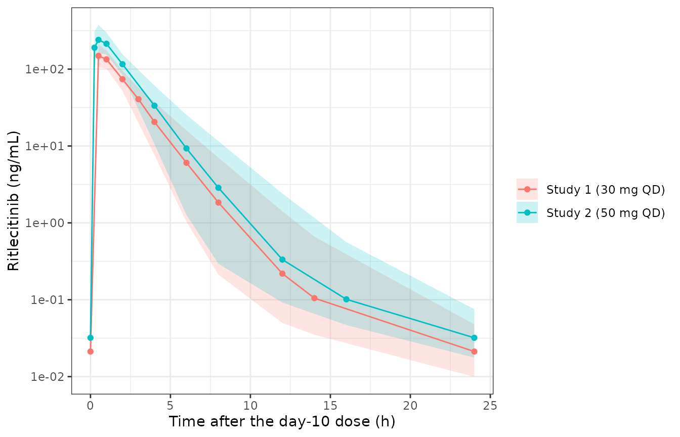
Simulated day-10 ritlecitinib plasma concentrations (median and 90% interval of individual predictions, 200 in silico healthy participants per study) at the protocol sampling times.
Assumptions and deviations
-
Interim model. Purohit 2023 describes this as a
fit-for-purpose iteration of the ritlecitinib population PK model, used
before the final model was available. The final development models,
which replace the dose switch with a concentration-driven autoinhibition
of clearance and bioavailability, are packaged as the
Wojciechowski_2023_ritlecitinib_*models. -
Allometric scaling of Q/F and Vp/F. Supplementary
Text S1 (‘Structural Model Development’) says weight scaling was applied
to Q/F and Vp/F as well as CL/F and Vc/F, but the final-model control
stream (
Q = THETA(4),V3 = THETA(5)) and the ‘Final Model’ paragraph scale only CL/F and Vc/F. The control stream is followed. -
No absorption lag. The control stream carries
ALAG1 = THETA(6) + FED*THETA(8)with both THETAs0 FIX, so the lag is identically zero and is not coded. -
Food covariate. The control-stream flag is any
non-zero FOOD value, and the supplement states the effect was assessed
in participants with a recorded high-fat meal (the food-effect arm of
NCT02684760); participants without a recorded food status were grouped
with the fasted. It is therefore mapped to
FED_HIGHFAT. -
Dose switch.
DOSE_HIGHis defined on the total daily dose (TRT = DOSE*DFREQ > 100mg), so 100 mg BID is in the high group. -
Scale of the IIV rows (departure from the printed
label). Table B’s footnote calls the IIV rows variances, but
the maintainers read them as SDs (0.156 on CL/F, 0.280 on Vc/F) with a
correlation of 0.173, as printed in NONMEM’s correlation matrix. The
evidence is the paper’s own Table IV, which only this reading reproduces
(see Scale of the variability
rows). The magnitudes also agree with the healthy-participant IIV of
the later
Wojciechowski_2023_ritlecitinib_basemodel (SD 0.201 on CL/F and 0.113 on Vc/F), and with the 16% CV of AUC observed in the Study 1 healthy participants. The labelled reading would imply about 45% CV. -
Residual error. The residual-error rows are kept as
the labelled $SIGMA variances of the log-transformed-both-sides model;
expSdHvandexpSdRaare their square roots (0.407 and 0.927). The healthy-participant value is close to the 0.340 proportional residual SD of the Wojciechowski 2023 base model. - In silico cohorts. The paper drew fresh weights for every one of 1000 trials; here 200 participants per study are simulated once and the trials are resampled from them, which reproduces the trial-to-trial distribution of the geometric mean without simulating 8000 participants. The food state on dosing days 1-9 (non-fasting in the studies) is not stated for the simulation; all doses are simulated fasted, which only alters ka and has no material effect on day-10 exposure. The assay lower limit of quantification is not reported, so concentrations were not censored to zero as the paper did.