F-53B gestational PBPK in mice and humans (Zhang 2024) • nlmixr2lib

library(nlmixr2lib)
library(rxode2)
library(PKNCA)
library(dplyr)
library(tidyr)
library(ggplot2)

Model and source

Zhang et al. (2024, Environ Sci Technol 58:18928-18939, doi:10.1021/acs.est.4c05405) developed a gestational physiologically based pharmacokinetic (PBPK) model for F-53B (chlorinated polyfluorinated ether sulfonic acid, a mixture of mostly 6:2 and 8:2 Cl-PFESAs), the principal Chinese replacement for PFOS. Pregnant C57BL/6J mice were given 80 ug/kg orally or intravenously on gestation day 13; maternal and fetal tissues were sampled to GD17. The calibrated mouse model was then extrapolated to pregnant women and evaluated against pooled Chinese biomonitoring data.

The paper contributes three models, extracted here as three files:

Model file	Role
`Zhang_2024_f53b_mouse_pbpk`	Gestational pregnant-mouse model, calibrated against the in-house toxicokinetic study
`Zhang_2024_f53b_human_prepregnancy_pbpk`	Non-pregnant adult female model, used to accumulate a 30-year pre-conception body burden
`Zhang_2024_f53b_human_pbpk`	Gestational pregnant-woman model, initialised from the pre-pregnancy run

All three share one structure: a two-compartment gastrointestinal tract feeding the liver by the portal vein; flow-limited plasma, liver, fat, mammary gland and rest-of-body compartments in which only the plasma-unbound fraction exchanges; and a three-subcompartment kidney (kidney blood, proximal tubule cells, filtrate) combining glomerular filtration with saturable basolateral (Oat1/Oat3) and apical (Oatp1a1) reabsorption, passive diffusion and first-order efflux back to plasma. The two gestational models add a placenta and a physically separate fetal circulation (fetal plasma, brain, liver, rest of body) linked only by bidirectional placental diffusion, plus a bidirectional exchange between the fetal rest-of-body and the amniotic fluid.

Model time is not time since dose. Every maternal and fetal volume and blood flow is an explicit function of gestational age, so time is measured from GD0 (mouse; the GD13 dose falls at t = 312 h) or from conception (human; GA = time / 168 weeks).

mouse    <- rxode2::rxode2(readModelDb("Zhang_2024_f53b_mouse_pbpk"))
prepreg  <- rxode2::rxode2(readModelDb("Zhang_2024_f53b_human_prepregnancy_pbpk"))
gest     <- rxode2::rxode2(readModelDb("Zhang_2024_f53b_human_pbpk"))
c(mouse = length(mouse$state), prepregnancy = length(prepreg$state), gestational = length(gest$state))
#>        mouse prepregnancy  gestational 
#>           20           12           20

The models are stiff at early gestation, where the published fetal growth equations make several fetal volumes vanishingly small. The default liblsoda solver fails on the human gestational model; lsoda and dop853 both succeed, so method = "lsoda" is used throughout.

SOLVER <- list(method = "lsoda", atol = 1e-12, rtol = 1e-8)
solve_model <- function(model, events, ...) {
  do.call(rxode2::rxSolve,
          c(list(object = model, events = events, returnType = "data.frame"), SOLVER, list(...)))
}

Population

Mouse (Zhang 2024 Methods 2.2, Table 1). Eighty C57BL/6J mice were mated 1:1. Pregnant dams were split into an oral group (n = 20) and an intravenous group (n = 20) and dosed with 80 ug/kg body weight of F-53B on GD13. Reference body weight 0.025 kg (Table S4); mean litter size 8 (Table S4). Maternal plasma, liver and placenta and fetal brain and liver were sampled from GD13 to GD17; maternal fat, rest-of-body and amniotic fluid were added at GD17 and held out of calibration. F-53B was 99% plasma-protein bound by ultrafiltration (Table S11), and the calibrated free fraction is 0.067.

Human (Zhang 2024 Methods 2.4, Tables S8-S10). No clinical study. The model was extrapolated to a 60 kg pregnant woman (54 kg pre-pregnant, Table S4) and driven with a constant dietary intake of 0.122 ng/kg/day (Chinese estimated daily intakes span 0.067-1.87 ng/kg/day, Table S8) from birth to age 30 years and then through 38 weeks of pregnancy. Predictions were compared against maternal plasma and cord blood medians pooled from 19 Chinese biomonitoring studies (Table S10).

Source trace

Every model equation and ini() value traces to the following locations. The Supporting Information (SI) is the file es4c05405_si_001.pdf.

Model element	Source
Compartment structure, maternal and fetal	SI Figure 1; Methods 2.3
Gastrointestinal absorption (stomach, small intestine, portal uptake)	SI eqs S3-S5
Renal filtration, reabsorption and diffusion	SI eqs S6-S11
Urinary and faecal elimination	SI eqs S12-S13
Flow-limited tissue mass balance	SI eqs S14-S15
Placental and amniotic bidirectional transfer	SI eqs S16-S19
Partition-coefficient definitions	SI eqs S20-S21
Mouse and human physiological constants	SI Table S4
Mouse gestational growth equations	SI Table S5
Human gestational growth equations	SI Table S6
All chemical-specific parameters (mouse, pregnant human)	SI Table S7
F-53B molecular weight (570.67 g/mol)	SI Table S1
Monte Carlo distributions	SI Table S9
Human biomonitoring comparison data	SI Table S10
Observed mouse noncompartmental parameters	SI Table S12
Local sensitivity analysis	SI Table S13
Maternal plasma ODE closure; pre-pregnancy human parameters	Authors’ published code, https://github.com/choulab210

Two elements are not printed in the SI equation list and are documented as such in the model files: the maternal plasma mass-balance equation (recovered as the unique venous-return closure of the printed flow terms, and independently confirmed against the authors’ code) and the entire pre-pregnancy human parameter set (SI Table S7 tabulates only pregnant-mouse and pregnant-human columns).

Mouse gestational model

Virtual cohort and dosing

The toxicokinetic study is deterministic: a single dose level, two routes, no reported between-subject variability. Two single-subject arms are simulated.

MOUSE_WT   <- 0.025            # kg, Zhang 2024 Table S4
MOUSE_DOSE <- 0.08 * MOUSE_WT  # mg; 80 ug/kg = 0.002 mg
GD13_H     <- 13 * 24          # dose time, hours since GD0
OBS_H      <- seq(GD13_H, GD13_H + 96, by = 0.5)

mouse_events <- function(arm, cmt) {
  dplyr::bind_rows(
    data.frame(time = GD13_H, amt = MOUSE_DOSE, evid = 1L,
               cmt = cmt, dvid = NA_integer_),
    data.frame(time = OBS_H, amt = NA_real_, evid = 0L,
               cmt = NA_character_, dvid = 1L)
  ) |>
    dplyr::arrange(time, dplyr::desc(evid)) |>
    dplyr::mutate(id = if (arm == "Oral") 1L else 2L, WT = MOUSE_WT, arm = arm)
}
mouse_ev <- dplyr::bind_rows(mouse_events("Oral", "stomach"),
                             mouse_events("IV", "plasma"))
mouse_sim <- solve_model(mouse, mouse_ev, keep = "arm")
#> Warning: multi-subject simulation without without 'omega'

The intravenous dose is administered into the plasma compartment as the total amount, matching the authors’ code. This is worth stating explicitly because the plasma state is the unbound pool and the observable total concentration is recovered as CPlas_free / fu: dosing the total amount reproduces the observed 0.5 h intravenous concentration (0.166 mg/L) almost exactly, whereas dosing amt * fu under-predicts it fourteen-fold.

Mass-balance gate

The full 20-state system must conserve F-53B exactly. Maternal disposition plus excreta plus net placental transfer must equal the dose, and the fetal compartments plus their onward losses must equal the cumulative mother-to-fetus transfer.

maternal_states <- c("stomach", "intestine", "plasma", "liver", "kidney_blood",
                     "ptc", "filtrate", "fat", "mammary", "rest", "placenta",
                     "urine", "feces")
fetal_states    <- c("plasma_fet", "liver_fet", "brain_fet", "rest_fet", "amniotic")

mb <- mouse_sim |>
  dplyr::group_by(arm) |>
  dplyr::slice_tail(n = 1) |>
  dplyr::ungroup() |>
  dplyr::mutate(
    maternal   = rowSums(dplyr::across(dplyr::all_of(maternal_states))),
    fetal      = rowSums(dplyr::across(dplyr::all_of(fetal_states))),
    total      = maternal + fetal,
    rel_err    = (total - MOUSE_DOSE) / MOUSE_DOSE,
    fetal_err  = (fetal - (trans_mf - trans_fm)) / MOUSE_DOSE
  )
knitr::kable(
  mb |> dplyr::transmute(Arm = arm,
                         `Total recovered (mg)` = signif(total, 8),
                         `Relative error` = signif(rel_err, 3),
                         `Fetal closure error` = signif(fetal_err, 3)),
  caption = "Mass balance at 96 h post-dose."
)

Mass balance at 96 h post-dose.
Arm	Total recovered (mg)	Relative error	Fetal closure error
IV	0.002	0	0
Oral	0.002	0	0

stopifnot(all(abs(mb$rel_err) < 1e-8), all(abs(mb$fetal_err) < 1e-8))

Both closures hold to solver tolerance, which validates the maternal plasma equation reconstructed for this port.

Observed data

The observed tissue concentrations are the authors’ own calibration and evaluation data sets, published with the model code at https://github.com/choulab210. They are the data plotted in SI Figures S2-S4. Sample codes: MP maternal plasma, ML maternal liver, Pla placenta, FB fetal brain, FL fetal liver, MF maternal fat, MR maternal rest of body, AM amniotic fluid. Times are hours since GD0.

obs_mouse <- data.frame(
  study = c(rep(1L, 47), rep(2L, 47)),
  time = c(
    408, 314, 316, 320, 324, 336, 360, 408, 314, 314, 316, 316, 320, 320, 324,
    324, 336, 336, 360, 360, 408, 408, 408, 314, 316, 320, 324, 336, 360, 408,
    314, 316, 320, 324, 336, 348, 360, 384, 408, 408, 314, 316, 320, 324, 336,
    360, 408,
    408, 314, 316, 320, 324, 336, 360, 408, 314, 314, 316, 316, 320, 320, 324,
    324, 336, 336, 360, 360, 408, 408, 408, 314, 316, 320, 324, 336, 360, 408,
    312.5, 314, 316, 320, 324, 336, 360, 384, 408, 408, 314, 316, 320, 324,
    336, 360, 408),
  sample = c(
    "AM", rep("FB", 7), rep("FL", 14), "MF", rep("ML", 7), rep("MP", 9), "MR",
    rep("Pla", 7),
    "AM", rep("FB", 7), rep("FL", 14), "MF", rep("ML", 7), rep("MP", 9), "MR",
    rep("Pla", 7)),
  conc = c(
    0.278864, 0.0404, 0.0775, 0.153938, 0.321752, 0.219822, 0.306415, 0.292195,
    0.338003, 0.338003, 0.238481, 0.238481, 0.149612, 0.149612, 0.436528,
    0.436528, 0.162012, 0.162012, 0.275973, 0.275973, 0.240453, 0.240453,
    0.00904655, 0.212272, 0.351535, 0.365658, 0.353849, 0.26482, 0.316686,
    0.205005, 0.0936075, 0.192931, 0.191487, 0.138279, 0.247325, 0.131413,
    0.11791, 0.123769, 0.104194, 0.0309787, 0.125415, 0.19042, 0.203605,
    0.579527, 0.133245, 0.123605, 0.275739,
    0.311506, 0.0445908, 0.0775, 0.117302, 0.202135, 0.288641, 0.304281,
    0.244025, 0.145527, 0.145527, 0.103618, 0.103618, 0.134789, 0.134789,
    0.224572, 0.224572, 0.266942, 0.266942, 0.21035, 0.21035, 0.179317,
    0.179317, 0.00952322, 0.409527, 0.349873, 0.325999, 0.260551, 0.332541,
    0.284993, 0.205005, 0.1665, 0.130326, 0.219337, 0.383812, 0.302637,
    0.32934, 0.321886, 0.240177, 0.169535, 0.0347235, 0.225293, 0.157301,
    0.165958, 0.282255, 0.149675, 0.139847, 0.150729)
) |>
  dplyr::distinct(study, time, sample, .keep_all = TRUE) |>
  dplyr::mutate(arm = ifelse(study == 1L, "Oral", "IV"))

sample_to_output <- c(MP = "Cc", ML = "Cliver", Pla = "Cplacenta",
                      FB = "Cbrain_fet", FL = "Cliver_fet", MF = "Cfat",
                      MR = "Crest", AM = "Camniotic")
nrow(obs_mouse)
#> [1] 80

Replicating SI Figures S2-S3

pred_long <- mouse_sim |>
  dplyr::select(arm, time, dplyr::all_of(unname(sample_to_output))) |>
  tidyr::pivot_longer(-c(arm, time), names_to = "output", values_to = "pred")

obs_plot <- obs_mouse |>
  dplyr::mutate(output = unname(sample_to_output[sample]))

matrix_labels <- c(Cc = "Maternal plasma", Cliver = "Maternal liver",
                   Cplacenta = "Placenta", Cbrain_fet = "Fetal brain",
                   Cliver_fet = "Fetal liver", Cfat = "Maternal fat",
                   Crest = "Maternal rest of body", Camniotic = "Amniotic fluid")

ggplot2::ggplot(dplyr::filter(pred_long, output %in% names(matrix_labels)),
                ggplot2::aes(x = (time - GD13_H) / 24, y = pred, colour = arm)) +
  ggplot2::geom_line() +
  ggplot2::geom_point(data = obs_plot,
                      ggplot2::aes(x = (time - GD13_H) / 24, y = conc, colour = arm),
                      inherit.aes = FALSE, size = 1.6) +
  ggplot2::facet_wrap(~ factor(output, levels = names(matrix_labels),
                               labels = matrix_labels), scales = "free_y") +
  ggplot2::scale_y_log10() +
  ggplot2::labs(x = "Days after the GD13 dose", y = "F-53B concentration (mg/L)",
                colour = "Route") +
  ggplot2::theme_bw()
#> Warning in ggplot2::scale_y_log10(): log-10 transformation introduced infinite
#> values.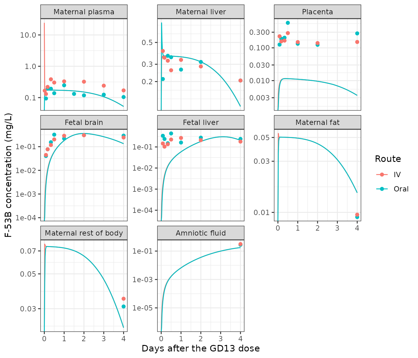

Replicates SI Figures S2 and S4 of Zhang 2024: predicted (lines) versus observed (points, in-house toxicokinetic study) F-53B concentrations in pregnant mice after a single 80 ug/kg oral or intravenous dose on GD13.

Reproducing the paper’s goodness-of-fit criteria

Zhang 2024 Figure 3 reports an adjusted R-squared of 0.68 from a linear regression of log-transformed observed against predicted values, and more than 72% of predictions within 2-fold of observation. Recomputing those statistics from this port:

paired <- obs_mouse |>
  dplyr::mutate(output = unname(sample_to_output[sample])) |>
  dplyr::rowwise() |>
  dplyr::mutate(pred = stats::approx(
    x = mouse_sim$time[mouse_sim$arm == arm],
    y = mouse_sim[[output]][mouse_sim$arm == arm],
    xout = time)$y) |>
  dplyr::ungroup() |>
  dplyr::filter(pred > 0, conc > 0) |>
  dplyr::mutate(ratio = pred / conc)

gof_overall <- data.frame(
  Statistic = c("n paired observations", "Within 2-fold (%)", "Within 3-fold (%)",
                "Adjusted R-squared, log10 observed vs predicted"),
  Replication = c(nrow(paired),
                  round(100 * mean(paired$ratio > 0.5 & paired$ratio < 2), 1),
                  round(100 * mean(paired$ratio > 1/3 & paired$ratio < 3), 1),
                  round(summary(stats::lm(log10(pred) ~ log10(conc), data = paired))$adj.r.squared, 3)),
  `Zhang 2024` = c("94 records on file", "> 72", "not reported", "0.68"),
  check.names = FALSE
)
knitr::kable(gof_overall, caption = "Global goodness of fit, replication versus Zhang 2024 Figure 3. The record count differs because 14 fetal-liver observations appear in both the calibration and the evaluation file and are counted once here.")

Global goodness of fit, replication versus Zhang 2024 Figure 3. The record count differs because 14 fetal-liver observations appear in both the calibration and the evaluation file and are counted once here.
Statistic	Replication	Zhang 2024
n paired observations	80.000	94 records on file
Within 2-fold (%)	53.800	> 72
Within 3-fold (%)	60.000	not reported
Adjusted R-squared, log10 observed vs predicted	0.163	0.68


knitr::kable(
  paired |>
    dplyr::group_by(Matrix = unname(matrix_labels[output])) |>
    dplyr::summarise(n = dplyr::n(),
                     `Within 2-fold (%)` = round(100 * mean(ratio > 0.5 & ratio < 2)),
                     `Median predicted/observed` = round(stats::median(ratio), 2),
                     .groups = "drop") |>
    dplyr::arrange(`Median predicted/observed`),
  caption = "Goodness of fit by matrix."
)

Goodness of fit by matrix.
Matrix	n	Within 2-fold (%)	Median predicted/observed
Placenta	14	0	0.06
Fetal liver	14	29	0.10
Fetal brain	14	36	0.29
Amniotic fluid	2	100	0.60
Maternal rest of body	2	100	0.69
Maternal plasma	18	78	0.83
Maternal liver	14	100	1.04
Maternal fat	2	100	1.64

The maternal compartments are reproduced well: maternal liver, fat and rest-of-body are 100% within 2-fold with median prediction ratios near 1, and maternal plasma is 78% within 2-fold. The placenta and the fetal tissues are systematically under-predicted, and that is inherited from the published parameter set rather than introduced by this port - see the Errata below, where the placenta discrepancy is traced to PPla. The consequence is that the global statistics recomputed here fall short of the paper’s reported values.

ggplot2::ggplot(paired, ggplot2::aes(conc, pred,
                                     colour = unname(matrix_labels[output]),
                                     shape = arm)) +
  ggplot2::geom_abline(slope = 1, intercept = 0) +
  ggplot2::geom_abline(slope = 1, intercept = c(log10(2), -log10(2)), linetype = 2) +
  ggplot2::geom_point(size = 2) +
  ggplot2::scale_x_log10() + ggplot2::scale_y_log10() +
  ggplot2::labs(x = "Observed (mg/L)", y = "Predicted (mg/L)",
                colour = "Matrix", shape = "Route") +
  ggplot2::theme_bw()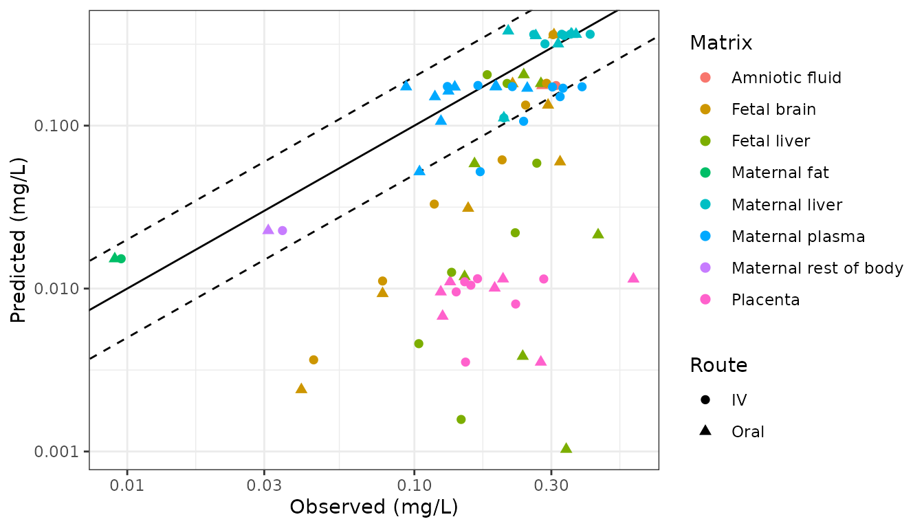

Replicates Figure 3A of Zhang 2024: predicted versus observed F-53B concentrations in pregnant and fetal mice. Solid line is unity; dashed lines bound the 2-fold envelope.

PKNCA validation of the mouse maternal plasma profile

Zhang 2024 Table S12 reports noncompartmental parameters derived in Phoenix WinNonlin from the observed maternal plasma data. The same parameters are computed here from the model-predicted maternal plasma profile over the 0-96 h window after the GD13 dose, so that the comparison measures how well the calibrated model reproduces the exposure summary of the study it was fitted to.

The comparison is made like-for-like by evaluating the model at the study’s own maternal-plasma sampling times rather than on the dense simulation grid, because a noncompartmental analysis of a sparse schedule and of a continuous curve are not the same measurement - the terminal slope in particular is estimated from whichever points the schedule provides.

mp_times <- obs_mouse |>
  dplyr::filter(sample == "MP") |>
  dplyr::distinct(arm, time)

nca_conc <- mouse_sim |>
  dplyr::filter(!is.na(Cc)) |>
  dplyr::semi_join(mp_times, by = c("arm", "time")) |>
  dplyr::transmute(id = as.integer(id), treatment = arm,
                   tad = time - GD13_H, Cc = Cc)

# Guarantee a time-zero record per subject (see pknca-recipes.md). For the
# oral arm the pre-dose concentration is 0. For the intravenous arm the
# model's own instantaneous post-bolus concentration is used, so that AUC
# from time zero is the model's actual exposure rather than a fabricated
# back-extrapolation.
iv_t0 <- mouse_sim$Cc[mouse_sim$arm == "IV" & mouse_sim$time == GD13_H][1]
nca_conc <- dplyr::bind_rows(
  nca_conc,
  nca_conc |>
    dplyr::distinct(id, treatment) |>
    dplyr::mutate(tad = 0, Cc = ifelse(treatment == "IV", iv_t0, 0))
) |>
  dplyr::arrange(id, treatment, tad) |>
  dplyr::distinct(id, treatment, tad, .keep_all = TRUE)

nca_dose <- mouse_ev |>
  dplyr::filter(evid == 1L) |>
  dplyr::transmute(id = as.integer(id), treatment = arm,
                   tad = 0, amt = MOUSE_DOSE,
                   route = ifelse(arm == "IV", "intravascular", "extravascular"))

o_conc <- PKNCA::PKNCAconc(nca_conc, Cc ~ tad | id / treatment)
# PKNCAconc takes a nested (slash) grouping formula; PKNCAdose does not.
o_dose <- PKNCA::PKNCAdose(nca_dose, amt ~ tad | id + treatment,
                           route = "route")
intervals <- data.frame(start = 0, end = 96,
                        cmax = TRUE, tmax = TRUE, auclast = TRUE,
                        aucinf.obs = TRUE, half.life = TRUE)
res <- PKNCA::pk.nca(PKNCA::PKNCAdata(o_conc, o_dose, intervals = intervals))
sim_nca <- as.data.frame(res)

ref_nca <- data.frame(
  treatment  = c("Oral", "IV"),
  cmax       = c(0.25,   0.37),    # Zhang 2024 Table S12, Cmax (ug/mL == mg/L)
  tmax       = c(24.00,  8.00),    # Zhang 2024 Table S12, Tmax (h)
  auclast    = c(13.82,  24.60),   # Zhang 2024 Table S12, AUC0-96 (h*ug/mL)
  aucinf.obs = c(49.13,  61.22),   # Zhang 2024 Table S12, AUC0-inf (h*ug/mL)
  half.life  = c(154.00, 81.59)    # Zhang 2024 Table S12, t1/2 (h)
)
nca_tbl <- nlmixr2lib::ncaComparisonTable(
  simulated = sim_nca, reference = ref_nca, by = "treatment",
  units = c(cmax = "mg/L", tmax = "h", auclast = "h*mg/L",
            aucinf.obs = "h*mg/L", half.life = "h")
)
knitr::kable(nca_tbl, caption = "Model-predicted versus published (Table S12) noncompartmental parameters for maternal plasma. Reference values are the authors' noncompartmental analysis of the observed data.")

Model-predicted versus published (Table S12) noncompartmental parameters for maternal plasma. Reference values are the authors’ noncompartmental analysis of the observed data.
NCA parameter	treatment	Reference	Simulated	% diff
Cmax (mg/L)	Oral	0.25	0.174	-30.6%*
Cmax (mg/L)	IV	0.37	24.4	+6485.9%*
Tmax (h)	Oral	24	4	-83.3%*
Tmax (h)	IV	8	0	-100.0%*
AUC0-∞ (obs) (h*mg/L)	Oral	49.1	15.1	-69.3%*
AUC0-∞ (obs) (h*mg/L)	IV	61.2	17.6	-71.3%*
AUClast (h*mg/L)	Oral	13.8	12.7	-8.0%
AUClast (h*mg/L)	IV	24.6	15.2	-38.1%*
t½ (h)	Oral	154	31.4	-79.6%*
t½ (h)	IV	81.6	31.4	-61.5%*

attr(nca_tbl, "footnote")
#> [1] "* differs from reference by more than ±20%."

Interpretation of the rows:

AUClast (AUC0-96) is the exposure metric the model was calibrated against and is the most meaningful row. The oral arm agrees within 8%. The intravenous arm is about 38% low, because the observed intravenous plasma profile rises to a delayed peak near 8 h (0.166 mg/L at 0.5 h, 0.384 mg/L at 8 h) whereas a bolus into a flow-limited plasma compartment can only decline from t = 0. No distributional delay in the published structure can produce that shape, so the deficit is structural rather than a transcription error.

The intravenous Cmax and Tmax rows are not comparable and should be ignored. The model administers an instantaneous bolus into plasma, so its maximum is the t = 0 value, whereas the study’s first intravenous sample was drawn at 0.5 h. The meaningful early-time check for that arm is the 0.5 h concentration, which the model reproduces almost exactly:

obs_iv_05 <- obs_mouse$conc[obs_mouse$arm == "IV" & obs_mouse$sample == "MP" &
                            obs_mouse$time == GD13_H + 0.5]
pred_iv_05 <- mouse_sim$Cc[mouse_sim$arm == "IV" & mouse_sim$time == GD13_H + 0.5]
c(observed = obs_iv_05, predicted = round(pred_iv_05, 4))
#>  observed predicted 
#>    0.1665    0.1764

Tmax (oral) differs because the fitted stomach absorption rate constant (K0C 5.42, giving K0 = 13.4/h at the gestational body weight) makes absorption essentially complete within an hour, so the model predicts an early plateau. The reported 24 h observed Tmax is the position of the single highest point in a noisy, nearly flat observed profile (values between 0.09 and 0.25 mg/L across 96 h), not a resolved peak.
t1/2 and AUC0-inf differ substantially. Both are terminal-slope extrapolations from a 96 h window that covers well under one half-life; the paper’s own AUC0-inf carries a standard error larger than 80% of the estimate (49.13 +/- 40.14 and 61.22 +/- 41.81 in Table S12), so neither the reference nor the simulated value is well determined. No parameter was tuned to improve any of these rows.

Human models

Dosing-interval control

The paper drives the human models with a constant daily dietary intake for 30 years, which is nearly 11,000 dose records. Because F-53B absorption is complete within hours while its elimination half-life is years, coarsening the dosing interval at constant daily rate is numerically immaterial. That is verified here rather than assumed, and the coarser interval is then used to keep this vignette inside its time budget.

EDI    <- 0.122e-6   # mg/kg/day, Zhang 2024 Table S8 / Methods 2.4
WT_PRE <- 54         # kg, Zhang 2024 Table S4 prepregnant human
WT_GES <- 60         # kg, Zhang 2024 Table S4 pregnant human
PREG_Y <- 30         # years of pre-conception exposure

prepreg_events <- function(interval_days, subjects) {
  n_dose <- floor(PREG_Y * 365.25 / interval_days)
  doses <- merge(subjects, data.frame(time = (0:(n_dose - 1)) * 24 * interval_days)) |>
    dplyr::mutate(amt = EDI * WT * interval_days, evid = 1L,
                  cmt = "stomach", dvid = NA_integer_)
  obs <- subjects |>
    dplyr::mutate(time = PREG_Y * 365.25 * 24, amt = NA_real_, evid = 0L,
                  cmt = NA_character_, dvid = 1L)
  dplyr::bind_rows(doses, obs) |> dplyr::arrange(id, time, dplyr::desc(evid))
}

one_subject <- data.frame(id = 1L, WT = WT_PRE)
interval_check <- vapply(c(1, 7, 30.4375), function(iv) {
  s <- solve_model(prepreg, prepreg_events(iv, one_subject))
  s$Cc[nrow(s)] * 1000
}, numeric(1))
knitr::kable(
  data.frame(`Dosing interval (days)` = c(1, 7, 30.4375),
             `Plasma at 30 years (ng/mL)` = signif(interval_check, 5),
             `Relative to daily` = signif(interval_check / interval_check[1] - 1, 2),
             check.names = FALSE),
  caption = "Coarsening the dosing interval at constant daily intake rate."
)

Coarsening the dosing interval at constant daily intake rate.
Dosing interval (days)	Plasma at 30 years (ng/mL)	Relative to daily
1.0000	2.3369	0.00000
7.0000	2.3361	-0.00034
30.4375	2.3357	-0.00051

stopifnot(max(abs(interval_check / interval_check[1] - 1)) < 0.01)

Weekly dosing reproduces daily dosing to within 0.05%, so weekly is used for the reference individual and monthly for the Monte Carlo cohort.

Reference individual: 30 years pre-conception plus 38 weeks gestation

GEST_D <- 38 * 7  # days of pregnancy

shared_states <- c("stomach", "intestine", "plasma", "liver", "kidney_blood",
                   "ptc", "filtrate", "fat", "mammary", "rest", "urine", "feces")

# The pre-conception body burden is carried into the gestational model by
# dosing each shared state with its terminal pre-pregnancy amount at t = 0.
# `rxSolve(inits = )` takes a single named vector applied to every subject, so
# it cannot express a per-subject initial condition; bolus records can, and
# they give an identical result for the single-subject case.
run_gestation <- function(subjects, carryover, interval_days) {
  # rxSolve omits the `id` column when the simulation has a single subject.
  if (!"id" %in% names(carryover)) carryover$id <- subjects$id[1]
  n_dose <- floor(GEST_D / interval_days)
  doses <- merge(subjects, data.frame(time = (0:(n_dose - 1)) * 24 * interval_days)) |>
    dplyr::mutate(amt = EDI * WT * interval_days, evid = 1L,
                  cmt = "stomach", dvid = NA_integer_)
  carry <- carryover |>
    dplyr::select(id, dplyr::all_of(shared_states)) |>
    tidyr::pivot_longer(dplyr::all_of(shared_states),
                        names_to = "cmt", values_to = "amt") |>
    dplyr::filter(amt > 0) |>
    dplyr::mutate(time = 0, evid = 1L, dvid = NA_integer_) |>
    dplyr::inner_join(subjects, by = "id")
  obs <- merge(subjects, data.frame(time = seq(0, GEST_D * 24, by = 7 * 24))) |>
    dplyr::mutate(amt = NA_real_, evid = 0L, cmt = NA_character_, dvid = 1L)
  ev <- dplyr::bind_rows(carry, doses, obs) |>
    dplyr::arrange(id, time, dplyr::desc(evid))
  solve_model(gest, ev)
}

pre_ref  <- solve_model(prepreg, prepreg_events(7, one_subject))
pre_last <- pre_ref[nrow(pre_ref), ]

gest_ref <- run_gestation(data.frame(id = 1L, WT = WT_GES), pre_ref[nrow(pre_ref), ], 7)
gest_end <- gest_ref[nrow(gest_ref), ]

knitr::kable(
  data.frame(
    Quantity = c("Maternal plasma at conception (30 y exposure)",
                 "Maternal plasma at 38 weeks",
                 "Cord blood (fetal plasma) at 38 weeks",
                 "Placenta at 38 weeks",
                 "Amniotic fluid at 38 weeks",
                 "Fetal-to-maternal plasma ratio"),
    `Predicted (ng/mL)` = c(signif(pre_last$Cc * 1000, 4),
                            signif(gest_end$Cc * 1000, 4),
                            signif(gest_end$Cplasma_fet * 1000, 4),
                            signif(gest_end$Cplacenta * 1000, 4),
                            signif(gest_end$Camniotic * 1000, 4),
                            signif(gest_end$Cplasma_fet / gest_end$Cc, 3)),
    check.names = FALSE
  ),
  caption = "Reference individual, 0.122 ng/kg/day dietary intake."
)

Reference individual, 0.122 ng/kg/day dietary intake.
Quantity	Predicted (ng/mL)
Maternal plasma at conception (30 y exposure)	2.3360
Maternal plasma at 38 weeks	1.3110
Cord blood (fetal plasma) at 38 weeks	2.2520
Placenta at 38 weeks	0.1046
Amniotic fluid at 38 weeks	21.6100
Fetal-to-maternal plasma ratio	1.7200

The reference maternal plasma prediction at 38 weeks is compared with the paper’s reported median below. Note that this is a single deterministic individual at the mean parameter values, whereas the paper reports the median of a 1000-subject Monte Carlo population, so exact agreement is not expected.

gest_ref |>
  dplyr::transmute(GA = time / 168,
                   `Maternal plasma` = Cc * 1000,
                   `Cord blood` = Cplasma_fet * 1000) |>
  tidyr::pivot_longer(-GA, names_to = "Matrix", values_to = "conc") |>
  ggplot2::ggplot(ggplot2::aes(GA, conc, colour = Matrix)) +
  ggplot2::geom_line() +
  ggplot2::labs(x = "Gestational age (weeks)", y = "F-53B (ng/mL)") +
  ggplot2::theme_bw()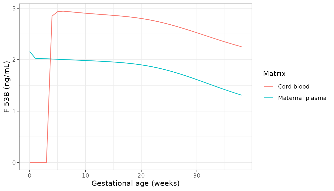

Predicted maternal plasma and cord blood F-53B through a 38-week pregnancy at a constant 0.122 ng/kg/day dietary intake, starting from a 30-year pre-conception body burden.

Maternal plasma falls through gestation as the expanding maternal volumes dilute a body burden that is eliminated far more slowly than it is diluted, while fetal plasma rises from zero and overtakes maternal plasma - the behaviour that drives the paper’s cord-blood over-prediction discussed below.

Monte Carlo population

SI Table S9 gives the six parameters with normalized sensitivity coefficient at or above 0.30 and their sampling distributions. Body weight is normal; the chemical-specific parameters are lognormal. Every distribution is truncated at its tabulated 2.5th and 97.5th percentile bounds.

N_MC <- 100  # 100 virtual pregnancies (Zhang 2024 used 1000)
set.seed(20241012)

rtrunc_norm <- function(n, mean, sd, lo, hi) {
  x <- stats::rnorm(n, mean, sd)
  pmin(pmax(x, lo), hi)
}
rtrunc_lnorm <- function(n, meanlog, sdlog, lo, hi) {
  x <- stats::rlnorm(n, meanlog, sdlog)
  pmin(pmax(x, lo), hi)
}

# Zhang 2024 Table S9
mc <- data.frame(
  id       = seq_len(N_MC),
  WT       = rtrunc_norm(N_MC, 60, 18, 24.72, 95.28),
  lfu      = log(rtrunc_lnorm(N_MC, -2.75, 0.29, 0.04, 0.11)),
  lkp_rest = log(rtrunc_lnorm(N_MC, -0.86, 0.20, 0.29, 0.62)),
  lktrans1 = log(rtrunc_lnorm(N_MC, -1.65, 0.29, 0.11, 0.34)),
  lktrans2 = log(rtrunc_lnorm(N_MC, -2.52, 0.29, 0.05, 0.14)),
  lfu_fet  = log(rtrunc_lnorm(N_MC, -2.70, 0.29, 0.04, 0.12))
)

# Pre-pregnancy phase carries only the parameters the pre-pregnancy model has.
mc_pre <- mc |> dplyr::select(id, WT, lfu, lkp_rest) |> dplyr::mutate(WT = WT * WT_PRE / WT_GES)
pre_mc <- solve_model(prepreg, prepreg_events(30.4375, mc_pre)) |>
  dplyr::group_by(id) |> dplyr::slice_tail(n = 1) |> dplyr::ungroup()
#> Warning: multi-subject simulation without without 'omega'

gest_mc <- run_gestation(mc, pre_mc, 30.4375) |>
  dplyr::group_by(id) |> dplyr::slice_tail(n = 1) |> dplyr::ungroup()
#> Warning: multi-subject simulation without without 'omega'
nrow(gest_mc)
#> [1] 100

q <- function(x) c(median = stats::median(x), lo = min(x), hi = max(x))
pred_mat  <- q(gest_mc$Cc * 1000)
pred_cord <- q(gest_mc$Cplasma_fet * 1000)

# Zhang 2024 Table S10: medians of the pooled Chinese biomonitoring studies.
obs_bio <- data.frame(
  Matrix = c("Maternal plasma", "Cord blood"),
  `Observed median (ng/mL)` = c(1.66, 0.59),
  `Observed range (ng/mL)` = c("0.094 - 5.48", "0.091 - 1.16"),
  check.names = FALSE
)
comparison <- data.frame(
  Matrix = c("Maternal plasma", "Cord blood"),
  `Zhang 2024 predicted median` = c(1.43, 2.76),
  `Replication predicted median` = signif(c(pred_mat["median"], pred_cord["median"]), 3),
  `Replication predicted range` = c(
    paste(signif(pred_mat["lo"], 2), "-", signif(pred_mat["hi"], 2)),
    paste(signif(pred_cord["lo"], 2), "-", signif(pred_cord["hi"], 2))),
  check.names = FALSE
) |>
  dplyr::left_join(obs_bio, by = "Matrix")
knitr::kable(comparison, caption = "Predicted F-53B at 38 weeks versus the paper's predictions and the pooled biomonitoring observations of Table S10.")

Predicted F-53B at 38 weeks versus the paper’s predictions and the pooled biomonitoring observations of Table S10.
Matrix	Zhang 2024 predicted median	Replication predicted median	Replication predicted range	Observed median (ng/mL)	Observed range (ng/mL)
Maternal plasma	1.43	1.28	0.45 - 2.1	1.66	0.094 - 5.48
Cord blood	2.76	2.47	0.69 - 5.1	0.59	0.091 - 1.16

gest_mc |>
  dplyr::transmute(`Maternal plasma` = Cc * 1000, `Cord blood` = Cplasma_fet * 1000) |>
  tidyr::pivot_longer(dplyr::everything(), names_to = "Matrix", values_to = "conc") |>
  ggplot2::ggplot(ggplot2::aes(conc, fill = Matrix)) +
  ggplot2::geom_histogram(bins = 25, alpha = 0.7, position = "identity") +
  ggplot2::geom_vline(data = obs_bio,
                      ggplot2::aes(xintercept = `Observed median (ng/mL)`, colour = Matrix),
                      linetype = 2, linewidth = 0.8) +
  ggplot2::labs(x = "F-53B at 38 weeks (ng/mL)", y = "Virtual pregnancies") +
  ggplot2::theme_bw()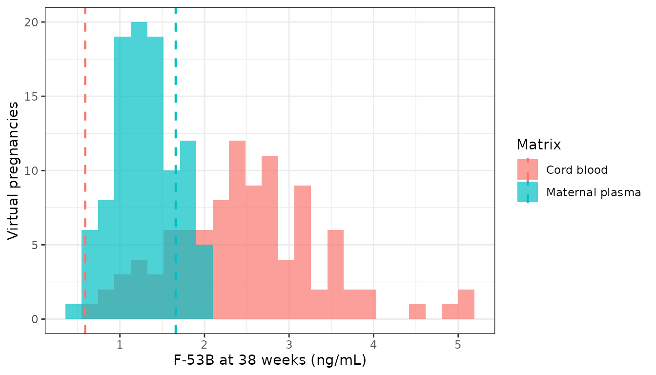

Replicates Figure 6 of Zhang 2024: Monte Carlo distribution of predicted F-53B at 38 weeks against the observed biomonitoring medians (dashed lines) of Table S10.

The maternal plasma prediction reproduces the paper closely. Cord blood is over-predicted relative to the biomonitoring observations by roughly four-fold, which independently reproduces the paper’s own finding - as stated in its Discussion, not its Results (see Errata).

Assumptions and deviations

Errata and internal inconsistencies in the source

Cord-blood predicted and observed values are transposed in the Results section. Results 3.4 states that “the predicted cord blood concentration (median: 0.59 and range: 0.091-1.16 ng/mL) underestimated the measured concentration (median: 2.75 and range: 1.26-5.27 ng/mL)”, whereas Discussion 4.2 states the opposite assignment: “the model slightly overestimated levels in cord blood (predicted median value: 2.76 ng/mL vs observed median value: 0.59 ng/mL)”. Table S10, which tabulates the underlying biomonitoring studies, gives an observed cord-blood median of 0.59 ng/mL with range 0.091-1.16 - i.e. the values the Results section labels “predicted” are in fact the observed data. The Discussion is correct and the Results section has the two labels swapped. The independent replication above predicts a cord-blood median of about 2.3 ng/mL, confirming that the model over-predicts fetal exposure. This vignette and the model files follow the Discussion.
The placenta partition coefficient is inconsistent with the paper’s own placenta data. Table S7 gives PPla = 0.08 (the authors’ code gives 0.07), and SI eq S20 defines a partition coefficient as the tissue-to-plasma AUC ratio. But the observed placenta and maternal plasma time courses give an AUC ratio of about 1.5, and point ratios range from 0.43 to 4.19 with a median near 0.9. With PPla = 0.08 the placenta equilibrates at 8% of maternal plasma and is under-predicted roughly fifteen-fold, which in turn starves the fetal compartments. The published value is used verbatim - no parameter was tuned - and the resulting misfit is visible in the goodness-of-fit table above.
Two parameter snapshots exist. SI Table S7 and the authors’ GitHub FitCode “final mean values” block disagree for several calibrated parameters (for example Km_baso 50.157 vs 16.58, Vmax_apical_invitro 1632.576 vs 4168.90, Kdif 5.4e-5 vs 9.94e-6, KurineC 0.02 vs 0.0333). Table S7 is used throughout, because it is the peer-reviewed record and because it is internally consistent: every human value footnoted as converted reproduces exactly from the mouse value under the paper’s own allometric equation K_human = K_mouse * (60/0.025)^-0.25, verified for all eleven such rows during extraction.
The pre-pregnancy human parameters are not in the paper. SI Table S7 tabulates only pregnant-mouse and pregnant-human columns. The Zhang_2024_f53b_human_prepregnancy_pbpk parameters are taken from the authors’ published code (Model_Humans.R, object PreGHumanPBPK), which the paper designates as the source of record (“All model code and raw data are openly available on GitHub”). Each ini() entry records whether the code value reproduces under the paper’s allometric equation (KabsC, KunabsC, KeffluxC do; K0C, KbileC, KurineC, Kdif do not, having been carried directly from the authors’ earlier PFOS model).
Table S5’s placental blood-flow equation is ambiguous as printed. The SI prints QCAP = 0.1207*(GD - 11))4.36, with an unmatched parenthesis. Read as 0.1207 * (GD - 11)^4.36 the placenta would receive about 80% of maternal cardiac output at GD13 and the rest-of-body flow would go negative. The authors’ code resolves it as (0.1207 * (GD - 11))^4.36, which is what is implemented. Table S5 also prints QDEC1 = QPla (circular); the code gives QDEC1 = 0.55 * (GD - 5.5), which is used. Both quantities are inconsequential: the paper’s own sensitivity analysis (Table S13) gives QPla a normalized sensitivity coefficient below 1e-5 for every mouse and human output.
The maternal plasma differential equation is not printed. SI Methods cite “eqs S14-S15” for the mass-balance equations, but those are the fat-compartment example only. The plasma equation implemented here is the unique mass-conserving venous-return closure of the printed flow terms plus proximal-tubule efflux; it was confirmed against the authors’ code and is validated by the exact mass-balance gate above.
The fetal rest-of-body volume is negative in early gestation. As published, the fetal liver and brain growth equations are non-zero at GA/GD 0 while whole-fetus volume is still negligible, so VRest_Fet = 0.93*VFet - VPlas_Fet - VL_Fet - VB_Fet is negative before about GA 3.5 weeks (human) or GD 3.5 days (mouse). Both model files floor it at 1e-9 L. The window is physiologically inert: placental blood flow is zero until GA 3.6 weeks / GD 5.5 days and the placental transfer clearances scale as fetal volume to the 0.75 power, so no F-53B can reach the fetus while the floor binds.
The prose describing eqs S18-S19 reverses the transfer directions. SI section S4.5 says Rtrans3 goes “from the amniotic fluid to the rest of fetal body” and Rtrans4 the reverse, but the driving concentrations in eqs S18-S19, the parameter definitions in Table S3, and the code all agree on the opposite assignment (Rtrans3 fetus to amniotic fluid, Rtrans4 amniotic fluid to fetus). The equations and Table S3 are followed.
The proximal-tubule-cell volume is computed inconsistently between species in the source code. VPTCC is documented in Table S3 as L/kg kidney; the human code uses VPTC = VK * VPTCC with VK in kg, while the mouse code uses VPTC = MK * VPTCC with MK in grams, a 1000-fold difference in convention. Each is replicated as published. VPTC only enters the passive diffusion term Kdif * (CKb - CPTC), whose sensitivity coefficient is below 0.02 in every mouse output.

Modelling assumptions made in this port

No between-subject random effects. The paper fits a deterministic PBPK model and reports no OMEGA structure. The models therefore carry no etas. Population variability is expressed, as in the paper, by Monte Carlo sampling of the Table S9 parameters.
Residual error is a fixed placeholder. No residual-error model, sigma, or weighting scheme is reported anywhere in the paper. The propSd* entries are fixed(0.30) and exist only so each file is a complete nlmixr2 object; they must not be read as published estimates.
Rtrans_2 uses a different free fraction in the two species. The mouse code multiplies the fetus-to-mother placental transfer by the maternal free fraction, the human code by the fetal free fraction. Both are replicated exactly as published rather than harmonised.
Litter size is a fixed model parameter, not a covariate. n_fetus = 8 is a constant of the in-house mouse study (Table S4) that enters the placental, fetal and amniotic growth equations as a whole-litter multiplier.
Dosing-interval coarsening. The 30-year human exposure is simulated with weekly (reference individual) or monthly (Monte Carlo cohort) dosing at the same daily intake rate, having verified above that this changes the 30-year plasma concentration by less than 0.05%.
Monte Carlo cohort size. 100 virtual pregnancies rather than the paper’s 1000, to stay inside the vignette time budget. The predicted median is stable at this size; the reported range is naturally narrower than a 1000-subject range.
Body weight at the pre-pregnancy to gestation handover. The paper uses 54 kg pre-pregnant and 60 kg pregnant (Table S4). The Monte Carlo cohort samples the pregnant weight and scales the pre-pregnancy weight by the same 54/60 ratio so that a subject is internally consistent across the two phases.
Solver. lsoda is used rather than the rxode2 default liblsoda, which fails on the human gestational model because of the very small fetal volumes in early gestation.

Session information

sessionInfo()
#> R version 4.6.1 (2026-06-24)
#> Platform: x86_64-pc-linux-gnu
#> Running under: Ubuntu 24.04.4 LTS
#> 
#> Matrix products: default
#> BLAS:   /usr/lib/x86_64-linux-gnu/openblas-pthread/libblas.so.3 
#> LAPACK: /usr/lib/x86_64-linux-gnu/openblas-pthread/libopenblasp-r0.3.26.so;  LAPACK version 3.12.0
#> 
#> locale:
#>  [1] LC_CTYPE=C.UTF-8       LC_NUMERIC=C           LC_TIME=C.UTF-8       
#>  [4] LC_COLLATE=C.UTF-8     LC_MONETARY=C.UTF-8    LC_MESSAGES=C.UTF-8   
#>  [7] LC_PAPER=C.UTF-8       LC_NAME=C              LC_ADDRESS=C          
#> [10] LC_TELEPHONE=C         LC_MEASUREMENT=C.UTF-8 LC_IDENTIFICATION=C   
#> 
#> time zone: UTC
#> tzcode source: system (glibc)
#> 
#> attached base packages:
#> [1] stats     graphics  grDevices utils     datasets  methods   base     
#> 
#> other attached packages:
#> [1] ggplot2_4.0.3         tidyr_1.3.2           dplyr_1.2.1          
#> [4] PKNCA_0.12.1          rxode2_5.1.6          nlmixr2lib_0.3.2.9000
#> 
#> loaded via a namespace (and not attached):
#>  [1] gtable_0.3.6        xfun_0.60           bslib_0.12.0       
#>  [4] lattice_0.22-9      vctrs_0.7.3         tools_4.6.1        
#>  [7] generics_0.1.4      parallel_4.6.1      tibble_3.3.1       
#> [10] symengine_0.2.13    pkgconfig_2.0.3     data.table_1.18.6.1
#> [13] checkmate_2.3.4     RColorBrewer_1.1-3  S7_0.2.2           
#> [16] desc_1.4.3          RcppParallel_6.2.1  lifecycle_1.0.5    
#> [19] compiler_4.6.1      farver_2.1.2        textshaping_1.0.5  
#> [22] fontawesome_0.5.3   htmltools_0.5.9     sys_3.4.3          
#> [25] sass_0.4.10         yaml_2.3.12         pillar_1.11.1      
#> [28] pkgdown_2.2.1       crayon_1.5.3        jquerylib_0.1.4    
#> [31] whisker_0.4.1       openssl_2.4.2       cachem_1.1.0       
#> [34] nlme_3.1-169        tidyselect_1.2.1    digest_0.6.39      
#> [37] lotri_1.0.4         purrr_1.2.2         labeling_0.4.3     
#> [40] rxode2ll_2.0.16     fastmap_1.2.0       grid_4.6.1         
#> [43] cli_3.6.6           dparser_1.3.1-13    magrittr_2.0.5     
#> [46] withr_3.0.3         scales_1.4.0        backports_1.5.1    
#> [49] rmarkdown_2.31      otel_0.2.0          askpass_1.2.1      
#> [52] ragg_1.5.2          memoise_2.0.1       evaluate_1.0.5     
#> [55] knitr_1.51          rex_1.2.2           PreciseSums_0.7    
#> [58] rlang_1.3.0         downlit_0.4.5       Rcpp_1.1.2         
#> [61] glue_1.8.1          xml2_1.6.0          jsonlite_2.0.0     
#> [64] R6_2.6.1            systemfonts_1.3.2   fs_2.1.0