Model and source
- Citation: Park SM, Lee J, Seong SJ, Park JG, Gwon MR, Lim MS, Lee HW, Yoon YR, Yang DH, Kwon KI, Han S. Population pharmacokinetic and pharmacodynamic modeling of transformed binary effect data of triflusal in healthy Korean male volunteers: a randomized, open-label, multiple dose, crossover study. BMC Pharmacology and Toxicology 2014;15:75. doi:10.1186/2050-6511-15-75.
- Description: One-compartment population PK with first-order
metabolite-formation kinetics for the active triflusal metabolite
hydroxy-4-(trifluoromethyl) benzoic acid (HTB) in healthy Korean male
volunteers, with a binary probability PD model for inhibition of
platelet aggregation (IPA). Triflusal is an antiplatelet prodrug; only
HTB is measured analytically. NONMEM ADVAN2 TRANS2 is used by the source
paper – the canonical depot compartment carries triflusal and the
canonical first-order rate constant (here
lka) plays the role of the paper’s HTB formation rate constant kf (0.341 1/h). Apparent oral clearance CL/F (0.200 L/h at 71.65 kg) and apparent oral volume V/F (8.300 L at 71.65 kg) describe HTB disposition; F absorbs the unknown fraction of triflusal converted to HTB. Body weight is the only retained covariate and enters as a power on CL/F (exponent 0.845) and direct proportionality on V/F (exponent fixed to 1). PD endpoint is binary IPA = 1 when platelet aggregation < 74% else 0; the instantaneous probability of IPA is a sigmoid Hill function of HTB concentration, prob_ipa = Cc^gamma / (EC50^gamma + Cc^gamma), with EC50 = 84.9 ug/mL and gamma = 19.2 (BSV on gamma fixed to 0). The Hill exponent is very steep (quantal-like concentration-response). Parameter values from Park 2014 Table 2 Estimates column. - Article: https://doi.org/10.1186/2050-6511-15-75
Population
Park 2014 enrolled 38 healthy Korean adult male volunteers in a
randomized, open-label, multiple-dose, two-period, two-treatment,
comparative crossover study at Kyungpook National University Hospital
Clinical Trial Center (KNUH CTC) between August and September 2008. Four
subjects dropped out; data from the remaining 34 subjects (mean age 24.1
+/- 1.7 years, mean height 176.1 +/- 4.9 cm, mean weight 70.8 +/- 9.0
kg) were used to construct the population PK and PD models. Volunteers
were required to be within 20% of their ideal body weight per the
Devine-style formula IBW (kg) = (height_cm - 100) * 0.9 and
to pass routine physical and laboratory screening. Baseline demographics
are reported in Park 2014 Table 1.
The dosing regimen during each period was a single 900 mg oral loading dose of triflusal on Day 1 followed by a 600 mg/day maintenance dose (two 300 mg capsules once daily) from Day 2 through Day 9. Plasma HTB was sampled at 0, 24, 48, 96, 144, 168, 192, 192.5, 193, 194, 196, 199, 202, and 216 h after the first dose; platelet aggregation was assessed at the same times excluding the dense post-Day-9 sub-sampling. Population PK was fit to 476 HTB plasma concentrations and population PD to 340 platelet- aggregation observations.
The structured population metadata is available
programmatically via
readModelDb("Park_2014_triflusal")()$meta$population.
Source trace
| Equation / parameter | Value | Source location |
|---|---|---|
Structural PK form (d/dt(depot) = -ka * depot;
d/dt(central) = ka * depot - kel * central) |
n/a | Methods: Population PK modeling – “ADVAN2 TRANS2” (1-cmt with
first-order absorption); the paper’s k_f plays the role of
the canonical ka
|
kf (= lka canonical) |
0.341 1/h | Park 2014 Table 2 theta_3 (RSE 15.1%) |
CL/F (= lcl canonical) |
0.200 L/h at 71.65 kg | Park 2014 Table 2 theta_1 (RSE 2.7%) |
V/F (= lvc canonical) |
8.300 L at 71.65 kg | Park 2014 Table 2 theta_2 (RSE 2.7%) |
(WT/71.65)^0.845 weight effect on CL/F |
exponent 0.845 (estimated) | Park 2014 Table 2 theta_4 (RSE 17.4%) |
(WT/71.65)^1 weight effect on V/F |
exponent fixed at 1 | Park 2014 Table 2 V/F equation
V_d/F = theta_2 * (weight/71.65) (no separate exponent
reported) |
EC50 (= lec50 canonical) |
84.9 ug/mL | Park 2014 Table 2 theta_5 (RSE 4.0%) |
Hill exponent gamma (= lhill
canonical) |
19.2 | Park 2014 Table 2 theta_6 (RSE 22.4%) |
P(IPA) = Cc^gamma / (EC50^gamma + Cc^gamma) |
n/a | Methods: Population PK-PD model development, binary probability model equation |
| BSV on CL/F | 14.9% CV | Park 2014 Table 2 omega_1^2 (RSE 21.0%; shrinkage 0.6%) |
| BSV on V/F | 9.5% CV | Park 2014 Table 2 omega_2^2 (RSE 57.8%; shrinkage 40.2%) |
| BSV on k_f | 88.0% CV | Park 2014 Table 2 omega_3^2 (RSE 26.5%; shrinkage 10.5%) |
| BSV on EC50 | 21.8% CV | Park 2014 Table 2 omega_4^2 (RSE 28.4%; shrinkage 8.3%) |
| BSV on gamma | 0 (fixed) | Park 2014 Table 2 omega_5^2 (NE) |
| Proportional residual error | sigma^2 = 0.098 | Park 2014 Table 2 sigma^2 (RSE 6.5%; shrinkage 11.5%); propSd = sqrt(0.098) |
Virtual cohort
The published trial data are not available. We assemble a virtual cohort of 200 healthy male volunteers with weights drawn from a truncated normal distribution that matches the reported 70.8 +/- 9.0 kg (53.3 - 89.7 kg range) of Park 2014 Table 1.
set.seed(20140523L)

n_subjects <- 200L

cohort <- tibble::tibble(
  id = seq_len(n_subjects),
  WT = pmin(pmax(rnorm(n_subjects, mean = 70.8, sd = 9.0), 53.3), 89.7)
)

# Dosing: 900 mg loading at t=0, then 600 mg/day from Day 2 to Day 9.
dose_times <- c(0, seq(from = 24, to = 192, by = 24))
dose_amts  <- c(900, rep(600, length(dose_times) - 1L))

dose_events <- expand.grid(
  id   = cohort$id,
  idx  = seq_along(dose_times)
) |>
  dplyr::mutate(
    time = dose_times[idx],
    amt  = dose_amts[idx],
    evid = 1L,
    cmt  = "depot"
  ) |>
  dplyr::select(id, time, amt, evid, cmt) |>
  dplyr::left_join(cohort, by = "id")

# Observation times: a dense grid + the paper's specific PK sampling points
obs_times <- sort(unique(c(
  seq(0, 216, by = 0.5),
  c(0, 24, 48, 96, 144, 168, 192, 192.5, 193, 194, 196, 199, 202, 216)
)))

obs_events <- expand.grid(
  id   = cohort$id,
  time = obs_times
) |>
  dplyr::mutate(
    amt  = NA_real_,
    evid = 0L,
    cmt  = NA_character_
  ) |>
  dplyr::left_join(cohort, by = "id")

events <- dplyr::bind_rows(dose_events, obs_events) |>
  dplyr::arrange(id, time, dplyr::desc(evid))

stopifnot(!anyDuplicated(unique(events[, c("id", "time", "evid")])))
Simulation
mod <- readModelDb("Park_2014_triflusal")()

sim <- rxode2::rxSolve(mod, events = events, keep = c("WT")) |>
  as.data.frame()
For deterministic typical-value replication (e.g., reproducing the paper’s Css,min and accumulation factor exactly), the random effects are zeroed:
mod_typical <- mod |> rxode2::zeroRe()

events_typical <- events |> dplyr::filter(id == 1L)
events_typical$WT <- 71.65

sim_typical <- rxode2::rxSolve(mod_typical, events = events_typical) |>
  as.data.frame()
#> ℹ omega/sigma items treated as zero: 'etalcl', 'etalvc', 'etalka', 'etalec50'
Replicate published figures
Figure 2(a) – HTB concentration over time
Park 2014 Figure 2(a) shows individual and median HTB plasma concentration profiles across the multi-dose regimen. The simulated VPC below uses the 200-subject virtual cohort.
vpc_df <- sim |>
  dplyr::filter(time %in% c(0, 24, 48, 96, 144, 168, 192, 192.5, 193, 194,
                            196, 199, 202, 216)) |>
  dplyr::group_by(time) |>
  dplyr::summarise(
    Q05 = quantile(Cc, 0.05, na.rm = TRUE),
    Q50 = quantile(Cc, 0.50, na.rm = TRUE),
    Q95 = quantile(Cc, 0.95, na.rm = TRUE),
    .groups = "drop"
  )

ggplot(vpc_df, aes(time, Q50)) +
  geom_ribbon(aes(ymin = Q05, ymax = Q95), alpha = 0.25, fill = "steelblue") +
  geom_line(colour = "steelblue", linewidth = 0.8) +
  geom_point(colour = "steelblue") +
  labs(
    x = "Time after first dose (h)",
    y = "HTB plasma concentration (ug/mL)",
    title = "Figure 2(a) -- simulated HTB concentration over time",
    subtitle = "Median and 5th/95th percentile across 200 virtual subjects",
    caption = "Replicates Figure 2(a) of Park 2014. Sampling times match the paper."
  ) +
  theme_minimal()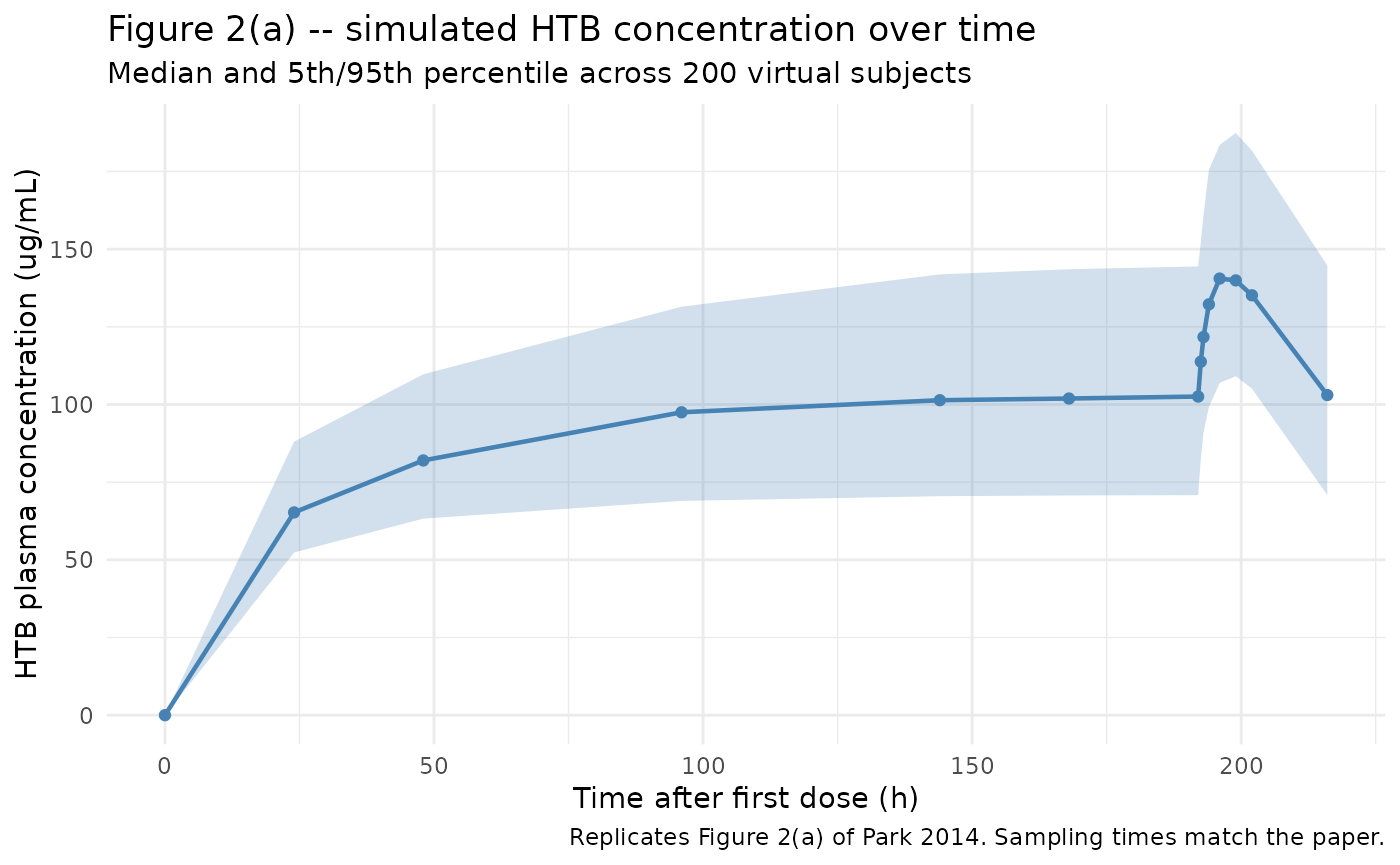
Figure 5(b) – predicted concentration vs probability of IPA
Park 2014 Figure 5(b) plots the predicted HTB concentration vs probability of IPA curve, with circles marking the model-predicted IPA probabilities at each individual PD sampling timepoint. The Hill exponent gamma = 19.2 is steep (quantal-like response).
conc_grid <- seq(0, 200, by = 0.5)
ec50 <- 84.9
hill <- 19.2
prob_curve <- conc_grid^hill / (ec50^hill + conc_grid^hill)

ggplot(data.frame(Cc = conc_grid, prob = prob_curve),
       aes(Cc, prob)) +
  geom_line(linewidth = 0.8, colour = "firebrick") +
  geom_vline(xintercept = ec50, linetype = "dashed", colour = "grey50") +
  geom_hline(yintercept = 0.5, linetype = "dashed", colour = "grey50") +
  annotate("text", x = ec50 + 2, y = 0.05,
           label = paste0("EC50 = ", ec50, " ug/mL"), hjust = 0) +
  labs(
    x = "HTB plasma concentration (ug/mL)",
    y = "Probability of IPA",
    title = "Figure 5(b) -- predicted concentration vs probability of IPA",
    caption = "Replicates Figure 5(b) of Park 2014."
  ) +
  theme_minimal()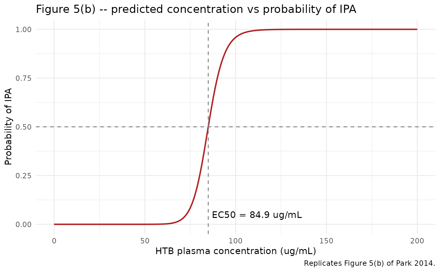
PKNCA validation
The paper reports two derived steady-state quantities under “Population PK modeling” / “Discussion”: Css,min = 103.5 ug/mL and accumulation factor = 2.26 (“estimated using the values of final population PK parameters”). PKNCA is used here on the typical-value simulation across the steady-state interval (the Day-8 to Day-9 window, the last full dosing interval before the dense intensive sampling) to extract Cmin, Cmax, AUC0-tau, and Cavg for comparison.
tau <- 24

# Use the typical-value simulation for the published-value comparison.
# rxSolve may drop the `id` column for single-subject simulations; add it
# back explicitly before passing to PKNCA.
sim_nca <- sim_typical |>
  dplyr::filter(!is.na(Cc), time >= 168, time <= 192) |>
  dplyr::mutate(id = 1L, treatment = "typical") |>
  dplyr::select(id, time, Cc, treatment)

conc_obj <- PKNCA::PKNCAconc(sim_nca,
                             Cc ~ time | treatment + id,
                             concu = "ug/mL",
                             timeu = "h")

dose_df <- dose_events |>
  dplyr::filter(id == 1L) |>
  dplyr::select(id, time, amt) |>
  dplyr::mutate(treatment = "typical")

dose_obj <- PKNCA::PKNCAdose(dose_df,
                             amt ~ time | treatment + id,
                             doseu = "mg")

intervals <- data.frame(
  start    = 168,
  end      = 192,
  cmin     = TRUE,
  cmax     = TRUE,
  tmax     = TRUE,
  auclast  = TRUE,
  cav      = TRUE
)

nca_res  <- PKNCA::pk.nca(PKNCA::PKNCAdata(conc_obj, dose_obj,
                                           intervals = intervals))

knitr::kable(
  as.data.frame(nca_res$result),
  digits = 3,
  caption = paste0(
    "PKNCA NCA over the Day-8 to Day-9 steady-state interval ",
    "(168 - 192 h post-first-dose) on the typical-value simulation."
  )
)| treatment | id | start | end | PPTESTCD | PPORRES | exclude | PPORRESU |
|---|---|---|---|---|---|---|---|
| typical | 1 | 168 | 192 | auclast | 2980.239 | NA | h*ug/mL |
| typical | 1 | 168 | 192 | cmax | 142.312 | NA | ug/mL |
| typical | 1 | 168 | 192 | cmin | 98.263 | NA | ug/mL |
| typical | 1 | 168 | 192 | tmax | 6.000 | NA | h |
| typical | 1 | 168 | 192 | cav | 124.177 | NA | ug/mL |
Comparison against published Css,min and accumulation factor
sim_cmin_ss <- min(sim_typical$Cc[sim_typical$time >= 168 &
                                  sim_typical$time <= 192])
# Accumulation factor (AUC basis) per closed-form for 1-cmt first-order:
# F_acc = 1 / (1 - exp(-kel * tau))
kel_typ <- 0.200 / 8.300
acc_factor_closed <- 1 / (1 - exp(-kel_typ * tau))

dplyr::tibble(
  Quantity = c("Css,min (ug/mL)", "AUC accumulation factor"),
  Published = c(103.5, 2.26),
  Simulated = round(c(sim_cmin_ss, acc_factor_closed), 2)
) |>
knitr::kable(caption = "Comparison against Park 2014 published values.")| Quantity | Published | Simulated |
|---|---|---|
| Css,min (ug/mL) | 103.50 | 98.26 |
| AUC accumulation factor | 2.26 | 2.28 |
Binary probability PD – post-processing
The PD endpoint in Park 2014 is the binary indicator IPA (1 =
inhibition, 0 = non-inhibition), dichotomised at platelet aggregation
< 74%. The model exposes prob_ipa as a deterministic
transform of Cc; binary draws are generated downstream from
prob_ipa. The chunk below reproduces Park 2014 Table 3
(observed vs predicted IPA counts at the PD sampling times) by averaging
the model-predicted prob_ipa across the virtual cohort.
table3_times <- c(0, 24, 48, 96, 144, 168, 192, 196, 202, 216)
n_sim <- length(unique(sim$id))

table3 <- sim |>
  dplyr::filter(time %in% table3_times) |>
  dplyr::group_by(time) |>
  dplyr::summarise(
    mean_prob_ipa  = mean(prob_ipa, na.rm = TRUE),
    expected_count = round(mean_prob_ipa * n_sim),
    expected_pct   = round(100 * mean_prob_ipa),
    .groups        = "drop"
  )

park2014_table3 <- dplyr::tibble(
  time = table3_times,
  paper_observed_pct  = c(3, 6, 32, 85, 74, 79, 88, 100, 100, 82),
  paper_predicted_pct = c(0, 6, 32, 74, 82, 88, 88, 100, 100, 88)
)

dplyr::inner_join(table3, park2014_table3, by = "time") |>
  dplyr::transmute(
    `Time (h)` = time,
    `Mean prob_ipa` = round(mean_prob_ipa, 3),
    `Simulated expected IPA (%)` = expected_pct,
    `Paper predicted IPA (%)`    = paper_predicted_pct,
    `Paper observed IPA (%)`     = paper_observed_pct
  ) |>
  knitr::kable(caption = paste0(
    "Park 2014 Table 3 -- observed vs predicted IPA counts. ",
    "Simulated expected IPA (%) is 100 * mean(prob_ipa) over the ",
    n_sim, "-subject virtual cohort."
))| Time (h) | Mean prob_ipa | Simulated expected IPA (%) | Paper predicted IPA (%) | Paper observed IPA (%) |
|---|---|---|---|---|
| 0 | 0.000 | 0 | 0 | 3 |
| 24 | 0.181 | 18 | 6 | 6 |
| 48 | 0.429 | 43 | 32 | 32 |
| 96 | 0.613 | 61 | 74 | 85 |
| 144 | 0.667 | 67 | 82 | 74 |
| 168 | 0.678 | 68 | 88 | 79 |
| 192 | 0.684 | 68 | 88 | 88 |
| 196 | 0.945 | 94 | 100 | 100 |
| 202 | 0.936 | 94 | 100 | 100 |
| 216 | 0.688 | 69 | 88 | 82 |
For a Bernoulli realization of the binary outcome:
Assumptions and deviations
- The PD endpoint is binary (IPA = 1 if platelet aggregation < 74%
else 0). The packaged model exposes the deterministic probability
prob_ipaas a derived quantity inmodel(); the model file declares onlyCcas the formal observation variable (with proportional residual error per Park 2014 Table 2). Binary realizations are drawn downstream viarbinom(n, 1, prob_ipa)– see the chunk above. This decision keeps the model file aligned with the nlmixr2 convention that observation variables carry standard residual-error families (add,prop,lnorm); the paper’s binary likelihood is encoded as a documented post-processing step rather than as an in-modeldbinom(prob, 1)call. - The cohort body-weight distribution is sampled from a truncated normal approximation of the reported mean +/- SD because the trial-level individual demographics are not publicly available.
- Race / ethnicity is set to 100% Asian to match the reported Korean cohort; no explicit race-effect covariate is in the model.
- The V/F covariate equation
V/F = theta_2 * (WT/71.65)is encoded withe_wt_vc <- fixed(1). The paper reports the equation without a separately estimated exponent, consistent with the authors’ Discussion statement that “V/F was directly proportional to weight (exponent = 1)”. - The Figure 1 caption lists PK sampling days (2, 3, 5, 7, 8, 9) but the Methods text “from Day 2 to 9” is the authoritative dosing schedule and is consistent with the paper’s reported steady-state Css,min = 103.5 ug/mL and AUC accumulation factor 2.26. The vignette and the model metadata reflect daily dosing across Day 2 - Day 9 inclusive.
- The paper’s
kf(first-order HTB formation rate constant) is encoded as the canonicallka. The math is identical to a 1-compartment first-order absorption model (NONMEM ADVAN2 TRANS2); the depot compartment carries triflusal and converts to HTB in central at rateka == kf. F (bioavailability) absorbs the unknown fraction of triflusal converted to HTB, so CL/F and V/F are apparent HTB-disposition parameters.