Pyrazinamide (Kim 2023)
Source:vignettes/articles/Kim_2023_pyrazinamide.Rmd
Kim_2023_pyrazinamide.RmdModel and source
- Citation: Kim R, Jayanti RP, Lee H, Kim H-K, Kang J, Park I-N, Kim J, Oh JY, Kim HW, Lee H, Ghim J-L, Ahn S, Long NP, Cho Y-S, Shin J-G; on behalf of the cPMTb. Development of a population pharmacokinetic model of pyrazinamide to guide personalized therapy: impacts of geriatric and diabetes mellitus on clearance. Front Pharmacol. 2023;14:1116226. doi:10.3389/fphar.2023.1116226
- Description: One-compartment population pharmacokinetic model with first-order absorption and first-order elimination for oral pyrazinamide in Korean adults with drug-susceptible tuberculosis (Kim 2023); lean body mass is an allometric covariate on CL/F and V/F (fixed exponents 0.75 and 1) and geriatric diabetes mellitus (age >= 70 years with diabetes mellitus) increases CL/F by 32%
- Article: https://doi.org/10.3389/fphar.2023.1116226
- Supplement (NONMEM control stream, subgroup sizes): https://www.frontiersin.org/articles/10.3389/fphar.2023.1116226/full#supplementary-material
Kim 2023 developed a one-compartment population PK model for oral pyrazinamide (PZA) in Korean tuberculosis patients, with the specific aim of testing whether advanced age interacts with comorbidities to alter PZA disposition. The headline finding is that patients who are simultaneously aged 70 years or older and diabetic have a 32% higher apparent oral clearance than everyone else – an interaction effect, since neither advanced age alone nor diabetes alone improved the fit.
Population
Kim 2023 enrolled 613 adults (> 18 years) with bacteriologically confirmed drug-susceptible tuberculosis from 18 hospitals in the Republic of Korea (cPMTb prospective cohort). Patients received a PZA-containing regimen – chiefly RHZE (85.8%) – for at least 2 weeks, dosed once daily at 20-30 mg/kg rounded to the nearest tablet size (500-2,000 mg; 67.2% of the training set received 1,500 mg). Non-adherent and non-steady-state patients were excluded.
The 613 patients were split at random 4:1 into a 488-patient training set (model development, the population the packaged model describes) and a 125-patient test set (external validation). Training-set baseline characteristics (Kim 2023 Table 1): median age 54.5 years (19-96), median total body weight 60.8 kg (28.8-95.3), median lean body weight 48.1 kg (23.1-63.79), 33.4% female, 11.27% with diabetes mellitus, and 3.9% with renal disease (eGFR <= 60 mL/min/1.73 m^2). Of the 613 enrolled, 110 were older than 70 years (median lean body weight 44.5 kg, range 23.14-58.77), of whom 23 were diabetic.
Sampling was deliberately sparse and randomised: blood was drawn at a random time 0-24 h after the last observed dose, typically one sample per outpatient and at least two samples per inpatient. PZA was quantified by validated HPLC-ESI-MS/MS over 2.0-80.0 ug/mL (LLOQ 2.0 ug/mL), with below-LLOQ values imputed as 1 ug/mL per Beal’s M5 method.
The same information is available programmatically via the model’s
population metadata
(readModelDb("Kim_2023_pyrazinamide")()$population).
Source trace
Every ini() entry in
inst/modeldb/specificDrugs/Kim_2023_pyrazinamide.R carries
an in-file comment naming its origin. They are collected here for
review. “Suppl. S1” is the NONMEM control stream reproduced in
Supplementary File S1 of the paper.
Note that Table 2 and Supplementary File S1 use different
theta indices for the same quantities. Table 2 numbers them
theta1 = CL/F, theta2 = geriatric-DM effect,
theta3 = Vd/F, theta4 = Ka; the control stream
numbers them THETA(1) = CL, THETA(2) = V,
THETA(3) = KA, THETA(4) = additive SD,
THETA(5) = proportional SD (fixed 0),
THETA(6)/THETA(7) = allometric exponents,
THETA(8) = geriatric-DM effect. The table below and the
model file’s comments always name which scheme they are quoting.
| Equation / parameter | Value | Source location |
|---|---|---|
| Structural model (1-cmt, first-order absorption and elimination) | n/a | Kim 2023 Results, “Development of a population PK model”; Suppl. S1
$SUBR ADVAN2 TRANS2
|
lka (Ka) |
1.49 1/h | Kim 2023 Table 2, Ka (1/h) = theta4
|
lcl (CL/F) |
4.49 L/h | Kim 2023 Table 2, CL/F (L/h) = theta1
|
lvc (V/F) |
44.2 L | Kim 2023 Table 2, Vd/F (L) = theta3
|
e_lbm_cl |
0.75 (fixed) | Kim 2023 Methods (“fixed exponents of 0.75 and 1”); Suppl. S1
$THETA (0.75 FIX)
|
e_lbm_vc |
1.0 (fixed) | Kim 2023 Methods; Suppl. S1 $THETA (1 FIX)
|
e_age_ge70_diab_cl |
0.32 | Kim 2023 Table 2,
CL/F; elder patient (>= 70 years old) with DM = theta1 x (1 + theta2), theta2
|
| Lean-body-weight reference | 48 kg | Suppl. S1 $PK:
TVCL = THETA (1) * (LBW/48)**(THETA(6)); rounded median of
the training set (48.1 kg, Kim 2023 Table 1) |
| Geriatric-diabetes indicator | AGE_GE70 * DIS_DIAB |
Suppl. S1 $PK: OLDDM1 = 0 /
IF (OLDDM.EQ.1) OLDDM1 = 1
|
etalcl |
0.01 | Kim 2023 Table 2, omega^2; CL/F (%) = 1 |
etalvc |
0.03 (fixed) | Kim 2023 Table 2, omega^2; Vd/F (%) = 3 (FIX); Suppl.
S1 $OMEGA (0.03 FIX)
|
etalka |
1.00 | Kim 2023 Table 2, omega^2; Ka (%) = 100 |
addSd |
3.41 ug/mL | Kim 2023 Table 2, Residual variability / Additive;
Suppl. S1 THETA (4)
|
propSd |
0 (fixed) | Suppl. S1 $THETA (0 FIX) = THETA(5), the
proportional term of
W = SQRT (THETA (4)**2 + THETA(5)**2 * IPRED**2)
|
Reading the IIV scale
Kim 2023 Table 2 labels its variability rows
omega^2; <parameter> (%), which is ambiguous on its
own – it could mean a variance, a CV%, or a variance expressed as a
percentage. The fixed V/F row settles it: Table 2 prints
3 (FIX) where Suppl. S1 $OMEGA carries the
literal (0.03 FIX). The table therefore reports
100 * omega^2, so the three IIV entries are
omega^2 = 0.01 (CL/F), 0.03 (V/F, fixed) and
1.00 (Ka). The Ka variance of 1.00 and its 32.7% shrinkage
are consistent with the paper’s own explanation that absorption-phase
sampling was sparse.
Virtual cohort
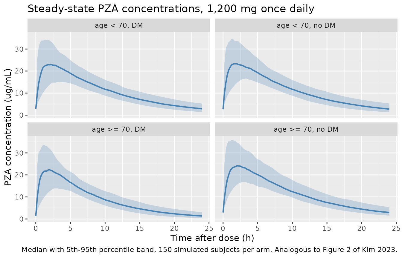
Original observed data are not publicly available. The cohort below mirrors the four subgroups Kim 2023 used for its Bayesian exposure comparison (Figure 4 and the “Bayesian estimation of PZA PK parameters” section): age < 70 vs >= 70 years, crossed with diabetes vs no diabetes. Doses are normalised to 1,200 mg once daily, as in the paper’s Figure 4.
Lean body weight is sampled per arm from a log-normal centred on the medians the paper reports – 48.1 kg for the training set as a whole (used for the age < 70 arms) and 44.5 kg for the > 70 year subgroup – and truncated to the observed range. This matters: because lean body weight scales CL/F allometrically, the lighter elderly patients have a lower CL/F, which is exactly the direction Kim 2023 reports for elderly non-diabetic patients.
set.seed(20230526)

dose_mg    <- 1200      # Kim 2023 Figure 4 normalises exposures to 1,200 mg
tau        <- 24        # once-daily dosing
n_dose     <- 7         # 7 daily doses reaches steady state (t1/2 ~ 6.8 h)
t_ss       <- tau * (n_dose - 1)   # start of the final (steady-state) interval
n_per_arm  <- 150       # <= 200 per arm

# Lean body weight: log-normal, truncated to the training-set range
# (23.1-63.79 kg, Kim 2023 Table 1).
lbm_sd_log <- 0.18
lbm_lo     <- 23.1
lbm_hi     <- 63.79

# `lbm_sd` is the log-scale SD of the lean-body-weight draw; pass 0 to pin every
# subject at `lbm_median` (used for the typical-value solve below).
make_arm <- function(n, arm, age_ge70, dis_diab, lbm_median, id_offset,
                     lbm_sd = lbm_sd_log) {
  subj <- tibble(
    id       = id_offset + seq_len(n),
    arm      = arm,
    AGE_GE70 = age_ge70,
    DIS_DIAB = dis_diab,
    LBM      = pmin(pmax(lbm_median * exp(rnorm(n, 0, lbm_sd)), lbm_lo), lbm_hi)
  )
  doses <- subj |>
    crossing(time = seq(0, tau * (n_dose - 1), by = tau)) |>
    mutate(amt = dose_mg, evid = 1L, cmt = "depot")
  obs <- subj |>
    crossing(time = seq(t_ss, t_ss + tau, by = 0.2)) |>
    mutate(amt = NA_real_, evid = 0L, cmt = "central")
  bind_rows(doses, obs) |> arrange(id, time, desc(evid))
}

events <- bind_rows(
  make_arm(n_per_arm, "age < 70, no DM",  0, 0, 48.1, id_offset =   0L),
  make_arm(n_per_arm, "age < 70, DM",     0, 1, 48.1, id_offset = 150L),
  make_arm(n_per_arm, "age >= 70, no DM", 1, 0, 44.5, id_offset = 300L),
  make_arm(n_per_arm, "age >= 70, DM",    1, 1, 44.5, id_offset = 450L)
)

# Disjoint IDs across arms are mandatory -- duplicate IDs silently merge.
stopifnot(!anyDuplicated(unique(events[, c("id", "time", "evid")])))

events |> count(arm, name = "rows")
#> # A tibble: 4 × 2
#>   arm               rows
#>   <chr>            <int>
#> 1 age < 70, DM     19200
#> 2 age < 70, no DM  19200
#> 3 age >= 70, DM    19200
#> 4 age >= 70, no DM 19200
Simulation
mod <- readModelDb("Kim_2023_pyrazinamide")

sim <- rxode2::rxSolve(
  mod,
  events = events,
  keep   = c("arm", "LBM", "AGE_GE70", "DIS_DIAB")
) |>
  as.data.frame() |>
  mutate(tad = time - t_ss)
#> ℹ parameter labels from comments will be replaced by 'label()'
A typical-value (no between-subject variability) solve is used to confirm the structural parameters reproduce Kim 2023 Table 2 exactly.
# lbm_sd = 0 pins every typical subject at the model's 48 kg lean-body-weight
# reference, so CL/F and V/F must come back as Kim 2023 Table 2's theta values.
typ_events <- bind_rows(
  make_arm(1, "age < 70, no DM",  0, 0, 48, id_offset = 1000L, lbm_sd = 0),
  make_arm(1, "age < 70, DM",     0, 1, 48, id_offset = 1001L, lbm_sd = 0),
  make_arm(1, "age >= 70, no DM", 1, 0, 48, id_offset = 1002L, lbm_sd = 0),
  make_arm(1, "age >= 70, DM",    1, 1, 48, id_offset = 1003L, lbm_sd = 0)
)

sim_typ <- rxode2::rxSolve(
  mod, events = typ_events, omega = NA, sigma = NA,
  keep = c("arm", "LBM")
) |>
  as.data.frame()

sim_typ |>
  group_by(arm) |>
  summarise(
    LBM     = first(LBM),
    `CL/F`  = first(cl),
    `V/F`   = first(vc),
    Ka      = first(ka),
    .groups = "drop"
  ) |>
  rename("Subgroup" = arm, "Lean body weight (kg)" = LBM,
         "CL/F (L/h)" = `CL/F`, "V/F (L)" = `V/F`, "Ka (1/h)" = Ka) |>
  knitr::kable(
    digits  = 3,
    caption = paste(
      "Typical-value parameters at the 48 kg lean-body-weight reference.",
      "Kim 2023 Table 2 gives CL/F = 4.49 L/h, V/F = 44.2 L, Ka = 1.49 1/h,",
      "and the Results text quotes CL/F = 5.9 L/h for geriatric diabetic",
      "patients (4.49 x 1.32 = 5.93)."
    )
)| Subgroup | Lean body weight (kg) | CL/F (L/h) | V/F (L) | Ka (1/h) |
|---|---|---|---|---|
| age < 70, DM | 48 | 4.490 | 44.2 | 1.49 |
| age < 70, no DM | 48 | 4.490 | 44.2 | 1.49 |
| age >= 70, DM | 48 | 5.927 | 44.2 | 1.49 |
| age >= 70, no DM | 48 | 4.490 | 44.2 | 1.49 |
Replicate published figures
# Replicates Figure 2 of Kim 2023 (prediction-corrected VPC): the distribution
# of PZA concentrations across one steady-state dosing interval. Kim 2023
# plots the 5th, 50th and 95th percentiles.
sim |>
  filter(!is.na(Cc)) |>
  group_by(arm, tad) |>
  summarise(
    Q05 = quantile(Cc, 0.05), Q50 = quantile(Cc, 0.50),
    Q95 = quantile(Cc, 0.95), .groups = "drop"
  ) |>
  ggplot(aes(tad, Q50)) +
  geom_ribbon(aes(ymin = Q05, ymax = Q95), alpha = 0.25, fill = "steelblue") +
  geom_line(colour = "steelblue", linewidth = 0.8) +
  facet_wrap(~arm) +
  labs(
    x = "Time after dose (h)", y = "PZA concentration (ug/mL)",
    title = "Steady-state PZA concentrations, 1,200 mg once daily",
    caption = paste(
      "Median with 5th-95th percentile band, 150 simulated subjects per arm.",
      "Analogous to Figure 2 of Kim 2023."
    )
  )
# Replicates Figure 4 of Kim 2023: AUC0-24, Cmax and CL/F by age / diabetes
# subgroup.
sim |>
  filter(!is.na(Cc)) |>
  group_by(arm, id) |>
  summarise(
    Cmax    = max(Cc),
    `CL/F`  = first(cl),
    AUC024  = sum(diff(tad) * (head(Cc, -1) + tail(Cc, -1)) / 2),
    .groups = "drop"
  ) |>
  pivot_longer(c(AUC024, Cmax, `CL/F`), names_to = "metric", values_to = "value") |>
  mutate(metric = recode(metric,
    AUC024 = "AUC0-24 (ug*h/mL)", Cmax = "Cmax (ug/mL)", `CL/F` = "CL/F (L/h)"
  )) |>
  ggplot(aes(arm, value, fill = arm)) +
  geom_boxplot(outlier.size = 0.4, show.legend = FALSE) +
  facet_wrap(~metric, scales = "free_y") +
  labs(
    x = NULL, y = NULL,
    title = "Exposure and clearance by age / diabetes subgroup (1,200 mg daily)",
    caption = "Replicates Figure 4 of Kim 2023."
  ) +
  theme(axis.text.x = element_text(angle = 30, hjust = 1))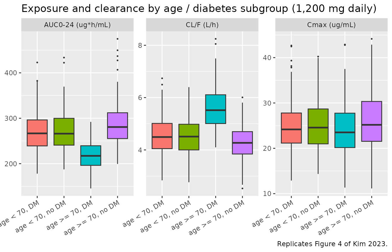
The model reproduces Kim 2023’s qualitative ordering: the geriatric diabetic arm has the highest CL/F and the lowest exposure, and among non-diabetic patients the elderly have higher exposure than the young because their lower lean body weight reduces CL/F allometrically. Note that the final covariate model assigns the same CL/F to all three non-geriatric-diabetic groups at equal lean body weight – the smaller differences Kim 2023 shows between those groups in Figure 4 come from individual Bayesian random effects, not from the covariate model.
PKNCA validation
Steady-state NCA over the final dosing interval (Recipe 3: AUC0-tau, Cmax, Cmin, Cavg).
sim_nca <- sim |>
  filter(!is.na(Cc)) |>
  select(id, time, Cc, arm)

conc_obj <- PKNCA::PKNCAconc(
  sim_nca, Cc ~ time | arm + id,
  concu = "ug/mL", timeu = "h"
)

dose_df <- events |>
  filter(evid == 1) |>
  select(id, time, amt, arm)

dose_obj <- PKNCA::PKNCAdose(
  dose_df, amt ~ time | arm + id,
  route = "extravascular", doseu = "mg"
)

intervals <- data.frame(
  start   = t_ss,
  end     = t_ss + tau,
  cmax    = TRUE,
  tmax    = TRUE,
  cmin    = TRUE,
  auclast = TRUE,
  cav     = TRUE
)

nca_res <- PKNCA::pk.nca(
  PKNCA::PKNCAdata(conc_obj, dose_obj, intervals = intervals)
)
as.data.frame(nca_res) |>
  filter(PPTESTCD %in% c("cmax", "tmax", "cmin", "auclast", "cav")) |>
  group_by(arm, PPTESTCD) |>
  summarise(median = median(PPORRES), .groups = "drop") |>
  pivot_wider(names_from = PPTESTCD, values_from = median) |>
  rename(
    "Subgroup"           = arm,
    "AUC0-24 (ug*h/mL)"  = auclast,
    "Cavg (ug/mL)"       = cav,
    "Cmax (ug/mL)"       = cmax,
    "Cmin (ug/mL)"       = cmin,
    "Tmax (h)"           = tmax
  ) |>
knitr::kable(digits = 2, caption = "Simulated steady-state NCA (medians of 150 subjects per arm), 1,200 mg once daily.")| Subgroup | AUC0-24 (ug*h/mL) | Cavg (ug/mL) | Cmax (ug/mL) | Cmin (ug/mL) | Tmax (h) |
|---|---|---|---|---|---|
| age < 70, DM | 266.68 | 11.11 | 24.17 | 2.88 | 1.8 |
| age < 70, no DM | 266.05 | 11.09 | 24.57 | 2.74 | 1.8 |
| age >= 70, DM | 217.21 | 9.05 | 23.52 | 1.36 | 1.6 |
| age >= 70, no DM | 280.68 | 11.69 | 25.18 | 2.95 | 2.0 |
Mass-balance check
At steady state under linear one-compartment kinetics, AUC over one
dosing interval must equal Dose / (CL/F) exactly, whatever
the absorption model. This is an internal consistency check on the
packaged model that requires no published number.
sim_typ |>
  filter(!is.na(Cc)) |>
  mutate(tad = time - t_ss) |>
  group_by(arm) |>
  summarise(
    `AUC0-24 (trapezoid)` = sum(diff(tad) * (head(Cc, -1) + tail(Cc, -1)) / 2),
    `Dose / (CL/F)`       = dose_mg / first(cl),
    .groups = "drop"
  ) |>
  mutate(`Ratio` = `AUC0-24 (trapezoid)` / `Dose / (CL/F)`) |>
  rename("Subgroup" = arm) |>
knitr::kable(digits = 3, caption = "Steady-state AUC0-24 equals Dose/(CL/F) for the typical subject in every subgroup.")| Subgroup | AUC0-24 (trapezoid) | Dose / (CL/F) | Ratio |
|---|---|---|---|
| age < 70, DM | 267.126 | 267.261 | 0.999 |
| age < 70, no DM | 267.126 | 267.261 | 0.999 |
| age >= 70, DM | 202.336 | 202.470 | 0.999 |
| age >= 70, no DM | 267.126 | 267.261 | 0.999 |
Comparison against published NCA
Kim 2023 reports median Bayesian-estimated AUC0-24 and Cmax per subgroup, normalised to a 1,200 mg dose, in the “Bayesian estimation of PZA PK parameters” section (visualised in Figure 4).
published <- tibble::tribble(
  ~arm,                ~cmax,  ~auclast,
  "age < 70, no DM",    23.88,   131.1,
  "age < 70, DM",       21.86,   123.2,
  "age >= 70, no DM",   25.92,   138.4,
  "age >= 70, DM",      21.28,    99.87
)

cmp <- nlmixr2lib::ncaComparisonTable(
  simulated     = nca_res,
  reference     = published,
  by            = "arm",
  params        = c("cmax", "auclast"),
  units         = c(cmax = "ug/mL", auclast = "ug*h/mL"),
  tolerance_pct = 20
)

knitr::kable(
  cmp,
  caption = "Simulated vs. published steady-state NCA at 1,200 mg once daily. * differs from reference by >20%.",
  align   = c("l", "l", "r", "r", "r")
)| NCA parameter | arm | Reference | Simulated | % diff |
|---|---|---|---|---|
| Cmax (ug/mL) | age < 70, no DM | 23.9 | 24.6 | +2.9% |
| Cmax (ug/mL) | age < 70, DM | 21.9 | 24.2 | +10.6% |
| Cmax (ug/mL) | age >= 70, no DM | 25.9 | 25.2 | -2.8% |
| Cmax (ug/mL) | age >= 70, DM | 21.3 | 23.5 | +10.5% |
| AUClast (ug*h/mL) | age < 70, no DM | 131 | 266 | +102.9%* |
| AUClast (ug*h/mL) | age < 70, DM | 123 | 267 | +116.5%* |
| AUClast (ug*h/mL) | age >= 70, no DM | 138 | 281 | +102.8%* |
| AUClast (ug*h/mL) | age >= 70, DM | 99.9 | 217 | +117.5%* |
Cmax agrees; AUC0-24 does not, and the discrepancy is in the paper. Every simulated Cmax is within about 11% of Kim 2023’s published median (within 3% for the two non-diabetic arms), so no Cmax row is starred. The simulated AUC0-24 values, however, are uniformly about 2.0-2.2x higher than the published ones, so all four AUC rows are starred.
This is an internal inconsistency in the source paper rather than a transcription error, and three independent arguments identify the published AUC0-24 column as the anomaly:
-
AUC0-24 = Dose/(CL/F) is an identity, not a fitted
quantity. With Table 2’s
CL/F = 4.49 L/h, a 1,200 mg daily dose gives1200 / 4.49 = 267 ug*h/mL. No absorption model, sampling scheme or Bayesian shrinkage can move that number to 131 ug*h/mL; only a CL/F near 9.2 L/h could, which is double what Table 2 reports. - The paper’s own Cmax values corroborate CL/F = 4.49 L/h. Solving the one-compartment oral model with Table 2’s parameters gives Cmax ~ 24.6 ug/mL at 1,200 mg, matching the published 23.88 ug/mL. A CL/F of 9.2 L/h would give Cmax ~ 19.7 ug/mL, which does not match the paper’s own Cmax.
- CL/F = 4.49 L/h agrees with the literature and with the paper’s Discussion, which compares its estimate against Rockwood 2016 (4.17 L/h), Mugabo 2019 (4.28 L/h) and Alsultan 2017 (5.06 L/h) – all near 4-5 L/h, none near 9 L/h.
The relative pattern across subgroups is nonetheless
reproduced well. Taking the covariate model at its two lean-body-weight
medians, it implies an elderly-non-diabetic / young-non-diabetic
exposure ratio of (48 / 44.5)^0.75 = 1.058 against the
published 138.4 / 131.1 = 1.056, and a geriatric-diabetic /
young-non-diabetic ratio of (48 / 44.5)^0.75 / 1.32 = 0.802
against the published 99.87 / 131.1 = 0.762. Only the absolute level of
the published AUC0-24 column is inconsistent. No parameter was tuned to
close the gap.
Assumptions and deviations
-
Lean body weight distribution. Kim 2023 reports
only the median and range of lean body weight, not its distribution.
Lean body weight is sampled here from a log-normal
(
sdlog = 0.18) truncated to the reported training-set range (23.1-63.79 kg), centred at 48.1 kg for the age < 70 arms and at the reported 44.5 kg elderly median for the age >= 70 arms. The paper does not report the lean-body-weight distribution separately for its diabetic strata, so diabetic and non-diabetic arms of the same age band share a distribution. - Subgroup sizes. Simulated arms are equal-sized (150 each) for a readable VPC. The real subgroups were very unequal (346 / 32 / 87 / 23 for young-non-DM / young-DM / elderly-non-DM / elderly-DM), so the published medians for the small diabetic strata carry much wider uncertainty than the simulated ones.
- Bayesian post-hoc vs prior-predictive. Kim 2023’s Figure 4 values are medians of individual Bayesian post-hoc estimates, each informed by that patient’s own observed concentration. The simulation here is a prior-predictive draw from the population model, so it cannot reproduce eta-driven differences between subgroups that the covariate model does not contain – notably the small young-DM vs young-non-DM difference, since diabetes alone is not a covariate in the final model.
- Steady state and dose. Doses are normalised to 1,200 mg once daily to match Figure 4; the actual cohort received 500-2,000 mg (67.2% at 1,500 mg). Seven daily doses are simulated and NCA is taken over the seventh interval, which is well past steady state for a ~6.8 h half-life.
-
Proportional residual error. Kept as
propSd = fixed(0)to preserve the provenance of Suppl. S1’s combined-error scaffold whose proportional coefficientTHETA(5)is declared(0 FIX). The active residual model is additive only, matching Kim 2023 Table 2. -
Covariates screened but not retained (total body
weight, continuous age, height, sex, feeding status, albumin, total
bilirubin, AST, ALT, eGFR-defined renal disease, liver disease, and the
>= 60 / >= 65 year age thresholds) are recorded in the model
file’s
covariatesDataExcludedmetadata rather thancovariateData, since none is referenced inmodel(). - All parameter values come from the paper’s Table 2 and Supplementary File S1. No value was taken from author correspondence, figure digitisation, or an upstream model.
Errata and internal inconsistencies in the source
-
Published AUC0-24 values are about 2.0-2.2x lower than
Dose/(CL/F)for every subgroup. See the comparison section above; the model follows Table 2 and Supplementary File S1, not the Figure 4 AUC values. - Patient count. The Abstract says “Data obtained from 610 TB patients”, but the Results and Table 1 say 613 (488 training + 125 test = 613). The 613 figure is used here.
-
Geriatric-diabetic CL/F. The Abstract quotes 5.73
L/h (geriatric DM) and 4.50 L/h (others), whereas Table 2 gives
theta1 = 4.49withtheta2 = 0.32, i.e. 4.49 and 4.49 x 1.32 = 5.93 L/h – the values the Results text quotes as 4.49 and 5.9 L/h. The model uses the Table 2 / Supplementary File S1 parameterisation, per the standing rule that the printed equation takes precedence over prose. - Young non-diabetic subgroup size. The Results text says 344 patients; Supplementary File S2 says 346, which is the value that makes the subgroups sum to the 488-patient training set (32 + 346 + 23 + 87 = 488). The supplement’s 346 is used here.
-
Table 2
%RSEfor the Ka variance is printed as(1), an implausibly small relative standard error for a variance whose point estimate is 1.00 and whose bootstrap interval is degenerate. Only the point estimate is needed for the model file, so this does not affect the implementation.