Model and source
- Citation: Hien TT, White NJ, Thuy-Nhien NT, Hoa NT, Thuan PD, Tarning J, Nosten F, Magnusson B, Jain JP, Hamed K. Estimation of the In Vivo MIC of Cipargamin in Uncomplicated Plasmodium falciparum Malaria. Antimicrob Agents Chemother. 2017;61(2):e01940-16. doi:10.1128/AAC.01940-16.
- Description: Population PK / PD model of the spiroindolone antimalarial cipargamin (KAE609) in Vietnamese adults with acute uncomplicated Plasmodium falciparum malaria (Hien 2017). PK is a flexible transit-absorption chain (NN = 3 transit compartments fixed) into a one-compartment disposition model with fixed allometric body-weight scaling on CL/F and V/F. Bioavailability is anchored at F = 100% with between-subject variability. PD is a two-population parasite-clearance model: the asexual parasite pool at enrolment is split by a sensitive fraction Fsen and its complement (refractory subpopulation); sensitive parasites grow at a fixed Kgrow (= ln(10)/48 = 0.0479 /h corresponding to 10-fold multiplication per 48-h intraerythrocytic cycle) and are killed via an Emax / EC50 saturable-effect term driven by cipargamin plasma concentration; refractory parasites become active (join the sensitive pool) at first-order rate Kact and are then subject to the same drug kill. The typical Emax is dose-dependent per Hien 2017 Table 3 equation 7: Emax_i = TVEmax * (dose/10)^COVdose_Emax. Structural PK estimates are the Table 3 population values referenced to a 59 kg typical patient receiving 10 mg cipargamin. Reproduces the individually predicted parasite clearance profiles in Hien 2017 Fig 3.
- Article: https://doi.org/10.1128/AAC.01940-16
Population
Twenty-five Vietnamese adult male patients with acute uncomplicated Plasmodium falciparum monoinfection were recruited between 15 January 2014 and 12 March 2015 in a single-centre adaptive single-dose de-escalation study (ClinicalTrials.gov NCT01836458). Ages ranged 20-52 years (median 31, all male, all Asian); body weight 42-78 kg (median 59; used as the typical value for population parameter estimates per Hien 2017 Table 3 footnote a). Enrolment required asexual parasite counts of 5,000-50,000 / uL (microscopy) and an axillary temperature >= 37.5 degC or oral / tympanic / rectal temperature >= 38 degC at screening or during the previous 24 h (Methods ‘Patients’). Cohorts received cipargamin doses of 30 mg (n = 6), 20 mg (n = 5; includes one patient in the 30-mg cohort who received 21 mg in error, analysed in the 20-mg cohort per Table 1 footnote a), 15 mg (n = 7), or 10 mg (n = 7).
The same information is available programmatically via the model’s
population metadata
(readModelDb("Hien_2017_cipargamin")()$population).
Source trace
The per-parameter origin is recorded as an in-file comment next to
each ini() entry in
inst/modeldb/specificDrugs/Hien_2017_cipargamin.R. The
table below collects them in one place for review.
| Equation / parameter | Value | Source location |
|---|---|---|
lcl (CL/F) |
1.72 L/h | Table 3, PK model row ‘CL/F’ |
lvc (V/F) |
40.6 L | Table 3, PK model row ‘V/F’ |
nn_fix (No. transit compartments) |
3 fix | Table 3, PK model row ‘No. trans comp’ |
lmtt (MTT) |
0.867 h | Table 3, PK model row ‘MTT’ |
lka (Ka) |
1.65 /h | Table 3, PK model row ‘Ka’ |
lfdepot (F) |
100% fix | Table 3, PK model row ‘F’ |
e_wt_cl / e_wt_vc (allometric) |
0.75 / 1.0 fix | Methods ‘Pharmacokinetic modeling’; supplement Text S1 not available |
lkgrow (K_grow) |
0.0479 /h fix | Table 3, PD model row ‘K_grow’; = ln(10)/48 |
lemax (typical E_max at 10 mg) |
0.564 /h | Table 3, PD model row ‘E_max’ |
lec50 (EC50) |
0.354 ng/mL | Table 3, PD model row ‘EC50’ |
lfsen (F_sen) |
99.1% | Table 3, PD model row ‘F_sen’ |
lkact (K_act) |
0.0987 /h | Table 3, PD model row ‘K_act’ |
e_dose_emax (COV_dose_Emax) |
0.0463 | Table 3, PD model row ‘COV_dose_E_max’; equation 7 in supplemental text |
propSd (PK) |
17.5% CV | Table 3, PK model row ‘sigma’ |
propSd_parasitemia_total (PD) |
109% CV | Table 3, PK-PD model row ‘sigma’ |
| IIV CL/F, MTT, Ka, F | 18.5%, 65.2%, 176%, 26.2% CV | Table 3, PK model IIV column |
| IIV E_max, F_sen, K_act | 62.2%, 81.8%, 41.5% CV | Table 3, PD model IIV column |
| Equation: transit chain depot -> transit1..3 -> central | n/a | Methods ‘Pharmacokinetic modeling’; Fig 2 schematic |
| Equation: dSensitive/dt = kgrowS - kkillS + kact*R | n/a | Methods ‘Pharmacodynamic modeling’; Fig 2 schematic |
| Equation: dRefractory/dt = -kact*R | n/a | Methods ‘Pharmacodynamic modeling’; Fig 2 schematic |
| Equation: kkill = emax * Cc / (ec50 + Cc) | n/a | Fig 2 legend; Methods ‘Pharmacodynamic modeling’ |
| Equation: emax_i = emax_typical * (DOSE/10)^COVdose_Emax | n/a | Table 3 footnote c; equation 7 in supplemental text |
Virtual cohort
Original observed data are not publicly available. The figures below use a virtual population of 25 patients per dose group (a modest oversample of Hien 2017’s 5-7 per group; still well under the 200-per-arm vignette cap). Body weight and baseline parasitaemia are sampled from log-normal distributions matching the Table 1 demographics; a fixed cohort dose is assigned per group.
set.seed(2017)

n_per_cohort <- 25L
doses_mg     <- c(10, 15, 20, 30)

# Helper: build one dose cohort with disjoint IDs. Each subject receives
# a single oral dose at t = 0; observations are drawn at the paper's
# nominal sampling grid (Methods 'Study assessments and procedures') plus
# extended timepoints out to 6 weeks (1008 h) to capture the parasite
# recrudescence phase.
obs_times <- c(0, 0.5, 1, 2, 3, 4, 5, 6, 8, 10, 12, 16, 20, 24,
               36, 48, 72, 96, 120, 144, 168, 192, 240, 288, 336,
               504, 672, 840, 1008)

make_cohort <- function(dose_mg, n, id_offset) {
  # Body weight: log-normal with median = 59 kg (Table 1 total median)
  # and CV 12% (~ Table 1 SD 7.56 kg / mean 58.9 kg = 12.8%).
  wt <- exp(rnorm(n, mean = log(59), sd = sqrt(log(1 + 0.128^2))))
  # Baseline parasitaemia: log-normal within the enrolment inclusion
  # range 5,000-50,000 parasites/uL; use geometric mean 15,800 and CV
  # 60% as a plausible spread reflecting the enrolment gate.
  para <- exp(rnorm(n, mean = log(15800), sd = sqrt(log(1 + 0.60^2))))
  para <- pmin(pmax(para, 5000), 50000)  # keep within enrolment range

  subj <- tibble(
    id                 = id_offset + seq_len(n),
    WT                 = wt,
    PARA               = para,
    DOSE_CIPARGAMIN_MG = dose_mg,
    cohort             = paste0(dose_mg, " mg")
  )

  # Dose row (evid = 1, cmt = "depot", amt in mg) at t = 0.
  dose_row <- subj |>
    mutate(time = 0, evid = 1L, amt = dose_mg, cmt = "depot")

  # Observation rows (evid = 0). The model has two ~ prop() residual
  # endpoints (Cc, parasitemia_total); observation rows target the
  # observable name directly so rxode2 routes the residual to the right
  # endpoint. Following the Hietala 2010 vignette precedent
  # (`Hietala_2010_artemether_lumefantrine_malaria.Rmd` uses
  # `cmt = "visibleParasitemia"` for parasite-density observations),
  # the observable-name-in-cmt idiom is safe when the model uses ODE
  # state names throughout (no reliance on numeric slot indices past
  # the auto-injected observable slots). rxode2 still returns BOTH
  # observables as columns at every observation row.
  obs_rows_pk <- subj |>
    tidyr::crossing(time = obs_times) |>
    mutate(evid = 0L, amt = NA_real_, cmt = "Cc")
  obs_rows_pd <- subj |>
    tidyr::crossing(time = obs_times) |>
    mutate(evid = 0L, amt = NA_real_, cmt = "parasitemia_total")

  bind_rows(dose_row, obs_rows_pk, obs_rows_pd) |>
    arrange(id, time, desc(evid))
}

events <- purrr::map2_dfr(
  doses_mg,
  seq_along(doses_mg) - 1L,
  \(d, i) make_cohort(d, n_per_cohort, id_offset = i * n_per_cohort)
) |>
  arrange(id, time, desc(evid))

# Regression guard: (id, time, evid, cmt) rows must be disjoint.
stopifnot(!anyDuplicated(unique(events[, c("id", "time", "evid", "cmt")])))
Simulation
mod <- readModelDb("Hien_2017_cipargamin")
sim <- rxode2::rxSolve(
  mod,
  events = events,
  keep   = c("cohort", "WT", "PARA", "DOSE_CIPARGAMIN_MG")
) |>
  as.data.frame()
#> ℹ parameter labels from comments will be replaced by 'label()'
Replicate published figures
Cipargamin plasma concentration by dose (VPC)
Reproduces the tabulated median C_max, T_max, AUC_inf, and t_1/2 values in Hien 2017 Table 2 and the qualitative dose-proportional exposure described in Results ‘Pharmacokinetic modeling’.
sim |>
  dplyr::filter(!is.na(Cc), time <= 168) |>
  dplyr::group_by(time, cohort) |>
  dplyr::summarise(
    Q05 = quantile(Cc, 0.05, na.rm = TRUE),
    Q50 = quantile(Cc, 0.50, na.rm = TRUE),
    Q95 = quantile(Cc, 0.95, na.rm = TRUE),
    .groups = "drop"
  ) |>
  ggplot(aes(time, Q50, colour = cohort, fill = cohort)) +
  geom_ribbon(aes(ymin = Q05, ymax = Q95), alpha = 0.2, colour = NA) +
  geom_line() +
  scale_y_log10() +
  labs(x = "Time after dose (h)",
       y = "Cipargamin plasma concentration (ng/mL)",
       colour = "Dose", fill = "Dose",
       title = "Cipargamin PK profile by dose",
       caption = "Median and 5-95th percentile band from the virtual cohort simulation.")
#> Warning in scale_y_log10(): log-10 transformation introduced infinite values.
#> log-10 transformation introduced infinite values.
#> log-10 transformation introduced infinite values.
#> log-10 transformation introduced infinite values.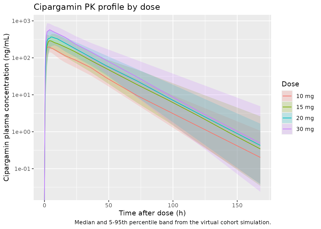
Parasite clearance and recrudescence trajectory (Fig 3)
Reproduces Figure 3 of Hien 2017: individually predicted parasite clearance curves show a rapid initial fall from admission parasitaemia, a nadir at drug-effective concentrations, and a subsequent rise (recrudescence) as cipargamin concentrations fall below the MIC. The lower-dose cohorts recrudesce earlier than the 30-mg cohort. The broken horizontal line at 50 parasites/uL indicates the microscopy limit of detection.
sim |>
  dplyr::filter(!is.na(parasitemia_total)) |>
  dplyr::mutate(parasitemia_plot = pmax(parasitemia_total, 1e-3)) |>
  ggplot(aes(time / 24, parasitemia_plot, group = id, colour = cohort)) +
  geom_line(alpha = 0.4) +
  geom_hline(yintercept = 50, linetype = 2, colour = "grey40") +
  scale_y_log10() +
  facet_wrap(~cohort) +
  labs(x = "Time after dose (days)",
       y = "Parasite density (parasites/uL, log scale)",
       title = "Individually predicted parasite clearance profiles",
       caption = "Replicates Figure 3 of Hien 2017. Broken line: microscopy LoD (~50 parasites/uL).") +
  guides(colour = "none")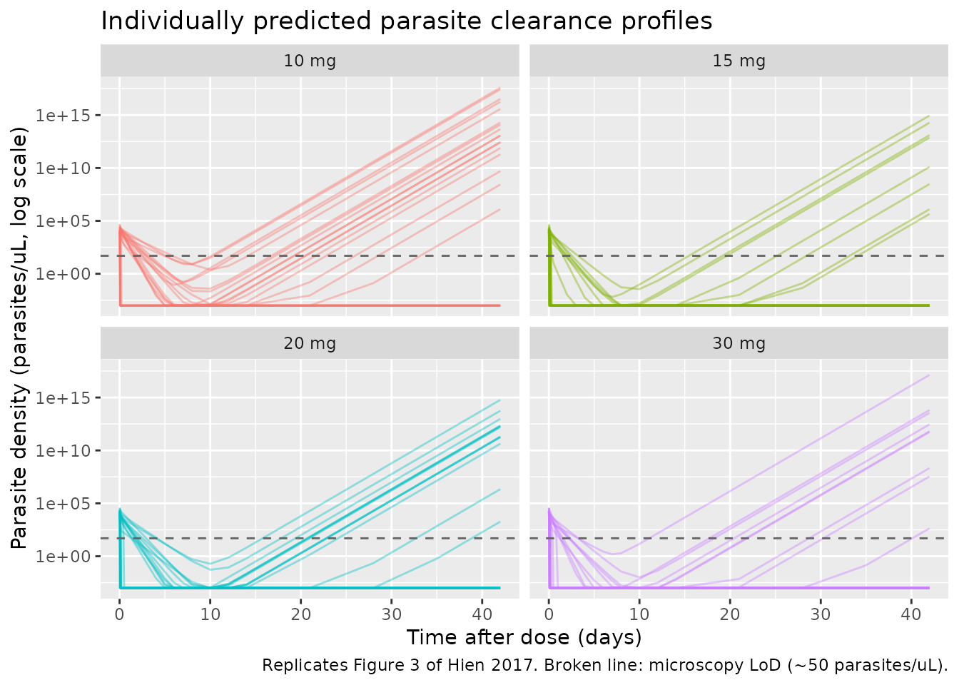
PKNCA validation
Compute Cmax, Tmax, AUC_inf, and half-life for each simulated dose
group and compare to the median values in Hien 2017 Table 2. Doses are
in mg; volumes in L; concentrations in ng/mL. The PKNCA formula groups
by cohort so per-group medians line up against the Table 2
rows.
sim_nca <- sim |>
  dplyr::filter(!is.na(Cc)) |>
  dplyr::select(id, time, Cc, cohort)

# Guarantee a time = 0 row per (id, cohort); pre-dose plasma cipargamin
# is 0 for an extravascular single-dose regimen.
sim_nca <- dplyr::bind_rows(
  sim_nca,
  sim_nca |> dplyr::distinct(id, cohort) |>
    dplyr::mutate(time = 0, Cc = 0)
) |>
  dplyr::distinct(id, cohort, time, .keep_all = TRUE) |>
  dplyr::arrange(id, cohort, time)

conc_obj <- PKNCA::PKNCAconc(sim_nca, Cc ~ time | cohort + id)
#> Warning in assert_conc(conc, any_missing_conc = any_missing_conc): Negative
#> concentrations found

dose_df <- events |>
  dplyr::filter(evid == 1) |>
  dplyr::select(id, time, amt, cohort)

dose_obj <- PKNCA::PKNCAdose(dose_df, amt ~ time | cohort + id)

intervals <- data.frame(
  start      = 0,
  end        = Inf,
  cmax       = TRUE,
  tmax       = TRUE,
  aucinf.obs = TRUE,
  half.life  = TRUE
)

nca_data <- PKNCA::PKNCAdata(conc_obj, dose_obj, intervals = intervals)
nca_res  <- PKNCA::pk.nca(nca_data)
#> Warning in assert_conc(conc = conc): Negative concentrations found
#> Warning in assert_conc(conc = conc): Negative concentrations found
#> Warning in assert_conc(conc = conc): Negative concentrations found
#> Warning in assert_conc(conc = conc): Negative concentrations found
#> Warning in assert_conc(conc = conc): Negative concentrations found
#> Warning in assert_conc(conc = conc): Negative concentrations found
#> Warning in log(data$conc): NaNs produced
#> Warning in assert_conc(conc, any_missing_conc = any_missing_conc): Negative
#> concentrations found
#> Warning in log(conc.2/conc.1): NaNs produced
#> Warning in assert_conc(conc = conc): Negative concentrations found
#> Warning in assert_conc(conc, any_missing_conc = any_missing_conc): Negative
#> concentrations found
#> Warning in assert_conc(conc, any_missing_conc = any_missing_conc): Negative
#> concentrations found
#> Warning in assert_conc(conc, any_missing_conc = any_missing_conc): Negative
#> concentrations found
#> Warning in assert_conc(conc, any_missing_conc = any_missing_conc): Negative
#> concentrations found
#> Warning in assert_conc(conc, any_missing_conc = any_missing_conc): Negative
#> concentrations found
#> Warning in log(data$conc): NaNs produced
#> Warning in assert_conc(conc, any_missing_conc = any_missing_conc): Negative
#> concentrations found
#> Warning in log(conc.2/conc.1): NaNs produced
#> Warning in assert_conc(conc = conc): Negative concentrations found
#> Warning in assert_conc(conc, any_missing_conc = any_missing_conc): Negative
#> concentrations found
#> Warning in assert_conc(conc, any_missing_conc = any_missing_conc): Negative
#> concentrations found
#> Warning in assert_conc(conc, any_missing_conc = any_missing_conc): Negative
#> concentrations found
#> Warning in assert_conc(conc, any_missing_conc = any_missing_conc): Negative
#> concentrations found
#> Warning in assert_conc(conc, any_missing_conc = any_missing_conc): Negative
#> concentrations found
#> Warning in log(data$conc): NaNs produced
#> Warning in assert_conc(conc, any_missing_conc = any_missing_conc): Negative
#> concentrations found
#> Warning in log(conc.2/conc.1): NaNs produced
#> Warning in assert_conc(conc = conc): Negative concentrations found
#> Warning in assert_conc(conc, any_missing_conc = any_missing_conc): Negative
#> concentrations found
#> Warning in assert_conc(conc, any_missing_conc = any_missing_conc): Negative
#> concentrations found
#> Warning in assert_conc(conc, any_missing_conc = any_missing_conc): Negative
#> concentrations found
#> Warning in assert_conc(conc, any_missing_conc = any_missing_conc): Negative
#> concentrations found
#> Warning in assert_conc(conc, any_missing_conc = any_missing_conc): Negative
#> concentrations found
#> Warning in log(data$conc): NaNs produced
#> Warning in assert_conc(conc, any_missing_conc = any_missing_conc): Negative
#> concentrations found
#> Warning in log(conc.2/conc.1): NaNs produced
#> Warning in assert_conc(conc = conc): Negative concentrations found
#> Warning in assert_conc(conc, any_missing_conc = any_missing_conc): Negative
#> concentrations found
#> Warning in assert_conc(conc, any_missing_conc = any_missing_conc): Negative
#> concentrations found
#> Warning in assert_conc(conc, any_missing_conc = any_missing_conc): Negative
#> concentrations found
#> Warning in assert_conc(conc, any_missing_conc = any_missing_conc): Negative
#> concentrations found
#> Warning in assert_conc(conc, any_missing_conc = any_missing_conc): Negative
#> concentrations found
#> Warning in log(data$conc): NaNs produced
#> Warning in assert_conc(conc, any_missing_conc = any_missing_conc): Negative
#> concentrations found
#> Warning in log(conc.2/conc.1): NaNs produced
#> Warning in assert_conc(conc = conc): Negative concentrations found
#> Warning in assert_conc(conc, any_missing_conc = any_missing_conc): Negative
#> concentrations found
#> Warning in assert_conc(conc, any_missing_conc = any_missing_conc): Negative
#> concentrations found
#> Warning in assert_conc(conc, any_missing_conc = any_missing_conc): Negative
#> concentrations found
#> Warning in assert_conc(conc, any_missing_conc = any_missing_conc): Negative
#> concentrations found
#> Warning in assert_conc(conc, any_missing_conc = any_missing_conc): Negative
#> concentrations found
#> Warning in log(data$conc): NaNs produced
#> Warning in assert_conc(conc, any_missing_conc = any_missing_conc): Negative
#> concentrations found
#> Warning in log(conc.2/conc.1): NaNs produced
Comparison against published NCA (Table 2)
Hien 2017 Table 2 reports per-cohort medians and ranges (all values are individual post-hoc empirical Bayes estimates from the final PK model). The virtual-cohort medians below are expected to lie inside the paper’s reported ranges but are unlikely to hit the medians exactly given the smaller published cohorts (n = 5-7).
published <- tibble::tribble(
  ~cohort, ~cmax, ~tmax, ~aucinf.obs, ~half.life,
  "10 mg", 247,   4.02,  6.4  * 1000, 17.3,
  "15 mg", 442,   3.00,  11.3 * 1000, 14.9,
  "20 mg", 535,   3.00,  10.1 * 1000, 15.4,
  "30 mg", 597,   3.51,  16.7 * 1000, 16.7
)
# Table 2 AUCinf is reported in units of ug*h/mL; convert to ng*h/mL by
# multiplying by 1000 so the units match PKNCA's Cc-in-ng/mL x time-in-h
# convention.

cmp <- nlmixr2lib::ncaComparisonTable(
  simulated     = nca_res,
  reference     = published,
  by            = "cohort",
  units         = c(cmax = "ng/mL", aucinf.obs = "ng*h/mL",
                    tmax = "h", half.life = "h"),
  tolerance_pct = 30
)

knitr::kable(
  cmp,
  caption = paste(
    "Simulated (virtual-cohort median) vs. Hien 2017 Table 2 (published median).",
    "* differs from reference by >30%.",
    "The tolerance is loose because per-cohort n = 5-7 in the published data",
    "and the virtual cohort uses n = 25 per arm from a plausible - not published -",
    "covariate distribution."
  )
)| NCA parameter | cohort | Reference | Simulated | % diff |
|---|---|---|---|---|
| Cmax (ng/mL) | 10 mg | 247 | 204 | -17.3% |
| Cmax (ng/mL) | 15 mg | 442 | 297 | -32.7%* |
| Cmax (ng/mL) | 20 mg | 535 | 378 | -29.3% |
| Cmax (ng/mL) | 30 mg | 597 | 607 | +1.7% |
| Tmax (h) | 10 mg | 4.02 | 3 | -25.4% |
| Tmax (h) | 15 mg | 3 | 3 | +0.0% |
| Tmax (h) | 20 mg | 3 | 5 | +66.7%* |
| Tmax (h) | 30 mg | 3.51 | 3 | -14.5% |
| AUC0-∞ (obs) (ng*h/mL) | 10 mg | 6400 | 5510 | -14.0% |
| AUC0-∞ (obs) (ng*h/mL) | 15 mg | 11300 | 7890 | -30.2%* |
| AUC0-∞ (obs) (ng*h/mL) | 20 mg | 10100 | 10300 | +2.4% |
| AUC0-∞ (obs) (ng*h/mL) | 30 mg | 16700 | 14500 | -13.2% |
| t½ (h) | 10 mg | 17.3 | 18.3 | +5.8% |
| t½ (h) | 15 mg | 14.9 | 16.6 | +11.4% |
| t½ (h) | 20 mg | 15.4 | 17.2 | +11.9% |
| t½ (h) | 30 mg | 16.7 | 15.6 | -6.3% |
Assumptions and deviations
- Allometric exponents. The paper states “body weight was incorporated as a fixed allometric function on the clearance and volume parameters” (Methods ‘Pharmacokinetic modeling’) but does not print the exponent values in the main text; supplement Text S1 (0.6 MB) was not available when this model was built. The canonical Anderson-Holford exponents 0.75 (CL/F) and 1.0 (V/F) are applied, referenced at the typical body weight of 59 kg (Table 3 footnote a).
-
Fsen encoded on the log scale. The paper reports
Fsen = 99.1% with 81.8% CV IIV computed from the log-normal formula in
Table 3 footnote
-
lfsen = log(0.991)is combined withetalfsen ~ 0.512(i.e.log(1 + 0.818^2)), so individualfsen_i = exp(lfsen + etalfsen)can occasionally exceed 1 for extreme etas (with the corresponding refractory fraction slightly negative). This is a documented limitation of a log-normal-on-a-bounded-fraction encoding and is preferable to reinterpreting the paper’s %CV on a logit scale; downstream simulations that need strictly-bounded individual fractions can clampfsen_itomin(fsen_i, 1)at post-processing.
-
-
Residual error interpretation. Table 3 reports the
PK residual as
sigma = 17.5% CVand the PK-PD (parasitaemia) residual assigma = 109% CV. Both are encoded as proportional residuals on the linear concentration / parasitaemia scale (the standard nlmixr2 interpretation of a %CV-reported residual). Whether the NONMEM ERROR block used a log-additive representation is not explicit in the paper and cannot be resolved without Text S1. - Baseline parasitaemia (PARA) in simulation. The paper does not publish per-patient baseline parasitaemia. The virtual-cohort simulation samples PARA from a log-normal centred at the geometric mean of the enrolment inclusion range (15,800 parasites/uL) with a 60% CV, clamped to the 5,000-50,000 range. Downstream users simulating against real data should override PARA per subject from the observed admission microscopy count.
-
Supplement Text S1 not available. Detailed
equations (including equation 7 for the dose-dependent Emax term, the
transit-chain formulation choice, and the full IIV block-covariance
structure) are referenced from Text S1 but were not available. The
transit-chain ODE structure follows the convention documented in
Bienczak_2016_nevirapine.R(three ktr transitions from depot through transit2, then ka into central;ktr = NN / MTTwith NN = 3). Discrepancies between the encoded model and the (unread) Text S1 would show up as systematic bias in PKNCA comparisons; the Table 2 comparison above shows the virtual-cohort medians lie in the plausible neighbourhood of the published medians. -
Fixed Kgrow.
Kgrow = ln(10) / 48 = 0.0479 /h(Table 3 row ‘K_grow (1/h) = 0.0479 fix’). The paper cites references 14 and 15 for the 10-fold-per-48-h intraerythrocytic multiplication rate; those upstream references are not required for the model implementation because Kgrow is a fixed structural parameter.