PEGylated asparaginase (Wurthwein 2021)
Source:vignettes/articles/Wurthwein_2021_pegasparaginase.Rmd
Wurthwein_2021_pegasparaginase.RmdModel and source
Wurthwein 2021 is the population PK model for PEGylated asparaginase
(PEG-ASNase) in the German and Czech part of the AIEOP-BFM ALL 2009
trial, covering the two induction doses and the single re-induction
dose. It is the direct predecessor of the four Wurthwein 2025 models
(Wurthwein_2025_pegasparaginase_*), which refit the same
structure to a larger and longer dataset. The two papers are packaged
separately because their estimates come from different fits.
- Citation: Wurthwein G, Lanvers-Kaminsky C, Siebel C, Gerss J, Moricke A, Zimmermann M, Stary J, Smisek P, Schrappe M, Rizzari C, Zucchetti M, Hempel G, Wicha SG, Boos J, on behalf of the AIEOP-BFM ALL 2009 Asparaginase Working Party. Population Pharmacokinetics of PEGylated Asparaginase in Children with Acute Lymphoblastic Leukemia: Treatment Phase Dependency and Predictivity in Case of Missing Data. Eur J Drug Metab Pharmacokinet. 2021;46(2):289-300. doi:10.1007/s13318-021-00670-8
- Article: https://doi.org/10.1007/s13318-021-00670-8
- Supplement: Electronic Supplementary Material 1 of the article. Section 2 documents the model building and Section 4 prints the complete NONMEM control stream of the Final Pharmacokinetic Model, which is the source of every equation in the model file.
mod <- rxode2::rxode(readModelDb("Wurthwein_2021_pegasparaginase"))
#> ℹ parameter labels from comments will be replaced by 'label()'
#> Warning: some etas defaulted to non-mu referenced, possible parsing error: etaiov_vc_1, etaiov_vc_2, etaiov_vc_3, etaiov_cl_1, etaiov_cl_2, etaiov_cl_3
#> as a work-around try putting the mu-referenced expression on a simple line
mod0 <- rxode2::zeroRe(mod)
#> Warning: some etas defaulted to non-mu referenced, possible parsing error: etaiov_vc_1, etaiov_vc_2, etaiov_vc_3, etaiov_cl_1, etaiov_cl_2, etaiov_cl_3
#> as a work-around try putting the mu-referenced expression on a simple line
Population
Children aged 1 to under 18 years with newly diagnosed acute lymphoblastic leukemia, treated in the AIEOP-BFM ALL 2009 trial (EudraCT 2007-004270-43, NCT01117441) at German and Czech sites. PEG-ASNase was given as a 2-hour intravenous infusion at 2500 U/m^2 (maximal absolute dose 3750 U) on protocol IA days 12 and 26 and, for non-high-risk patients only, on protocol II day 8, scheduled 18 weeks after the last induction dose. Activity was monitored 7 and 14 days after each dose.
The final model was fitted to the Final Dataset of 2545 patients and 11,486 samples (Section 4.1). Covariates were first selected on a Model Building Dataset (1374 patients, 6069 samples; median age 5.13 years, range 1.03-17.9; median BSA 0.78 m^2, range 0.41-2.42; 779 male / 595 female) and externally validated on a Testing Dataset (1253 patients, 5523 samples; median age 5.06 years; median BSA 0.77 m^2; 741 male / 512 female) (Table 1).
The model describes standard elimination only. Samples after a hypersensitivity reaction, samples indicating silent inactivation (activity below 100 U/L within 8 days and/or undetectable within 15 days) and pharmacologically implausible samples were excluded before fitting (Section 2.3).
The same information is available programmatically via
readModelDb("Wurthwein_2021_pegasparaginase")()$population.
Structural model
Asparaginase activity is carried by a chain of 14 serial
compartments sharing one serum volume V (Figure
1). Drug steps from compartment i to i+1 with
intercompartmental clearance Qtr, which the authors
interpret as stepwise de-PEGylation, and every compartment is eliminated
with the initial clearance CLinitial. In the authors’
earlier structural model the terminal compartment had its own induced
clearance CLinduced; this paper sets
CLinduced = Qtr (ESM Section 2, dOFV = 0.6), so every
compartment has the same total loss rate
(CLinitial + Qtr) / V. The assay measures total activity,
so the observation is the sum over all 14 states divided by
V (ESM Section 4 $ERROR).
Immediately after a dose the apparent clearance is
CLinitial. As mass moves down the chain it rises toward
CLinitial + Qtr, but slowly: the amounts are
Poisson-distributed in (Qtr/V) * t, and the terminal
compartment only fills once that exceeds about 13, i.e. after several
weeks. Over a 14-day interval the rise is modest, which is the curvature
the chain was built to reproduce.
The closed forms below use the typical child at the centring point
(BSA 0.79 m^2, male, age 5, first induction dose), where
V = 1.69 * 0.79 = 1.335 L,
CLinitial = 0.126 * 0.79 = 0.0995 L/day and
Qtr = 0.918 * 0.79 = 0.725 L/day (see “How the printed
values are quoted” below).
V0  <- 1.69 * 0.79
CL0 <- 0.126 * 0.79
Q0  <- 0.918 * 0.79
c(V = V0, CLinitial = CL0, Qtr = Q0)
#>         V CLinitial       Qtr
#>   1.33510   0.09954   0.72522
ev_ramp <- rxode2::et(amt = 2500 * 0.79, dur = 2 / 24, cmt = "central") |>
  rxode2::et(seq(0, 42, by = 0.05), cmt = "central") |>
  as.data.frame() |>
  mutate(BSA = 0.79, AGE = 5, SEXF = 0, OCC = 1)

ramp <- rxode2::rxSolve(mod0, ev_ramp, returnType = "data.frame") |>
  filter(time > 2 / 24) |>
  # Elimination rate = CLinitial * Ctotal + Qtr * transit13 / V, so
  #   CL_app = CLinitial + Qtr * (transit13 / V) / Cc.
  # With every compartment sharing the loss rate (ke + kt), the amounts are
  # Poisson in kt * t, giving the closed form
  #   CL_app = CLinitial + Qtr * dpois(13, kt * t) / ppois(13, kt * t).
  mutate(
    cl_app = CL0 + Q0 * (transit13 / V0) / Cc,
    cl_cf  = CL0 + Q0 * dpois(13, (Q0 / V0) * time) / ppois(13, (Q0 / V0) * time)
  )
#> ℹ omega/sigma items treated as zero: 'etalcl', 'etaiov_vc_1', 'etaiov_vc_2', 'etaiov_vc_3', 'etaiov_cl_1', 'etaiov_cl_2', 'etaiov_cl_3'

ggplot(ramp, aes(time)) +
  geom_line(aes(y = cl_app), linewidth = 0.9) +
  geom_line(aes(y = cl_cf), colour = "firebrick", linetype = "dashed") +
  geom_hline(yintercept = CL0, linetype = "dotted") +
  labs(x = "Days after dose", y = "Apparent clearance (L/day)") +
  theme_bw()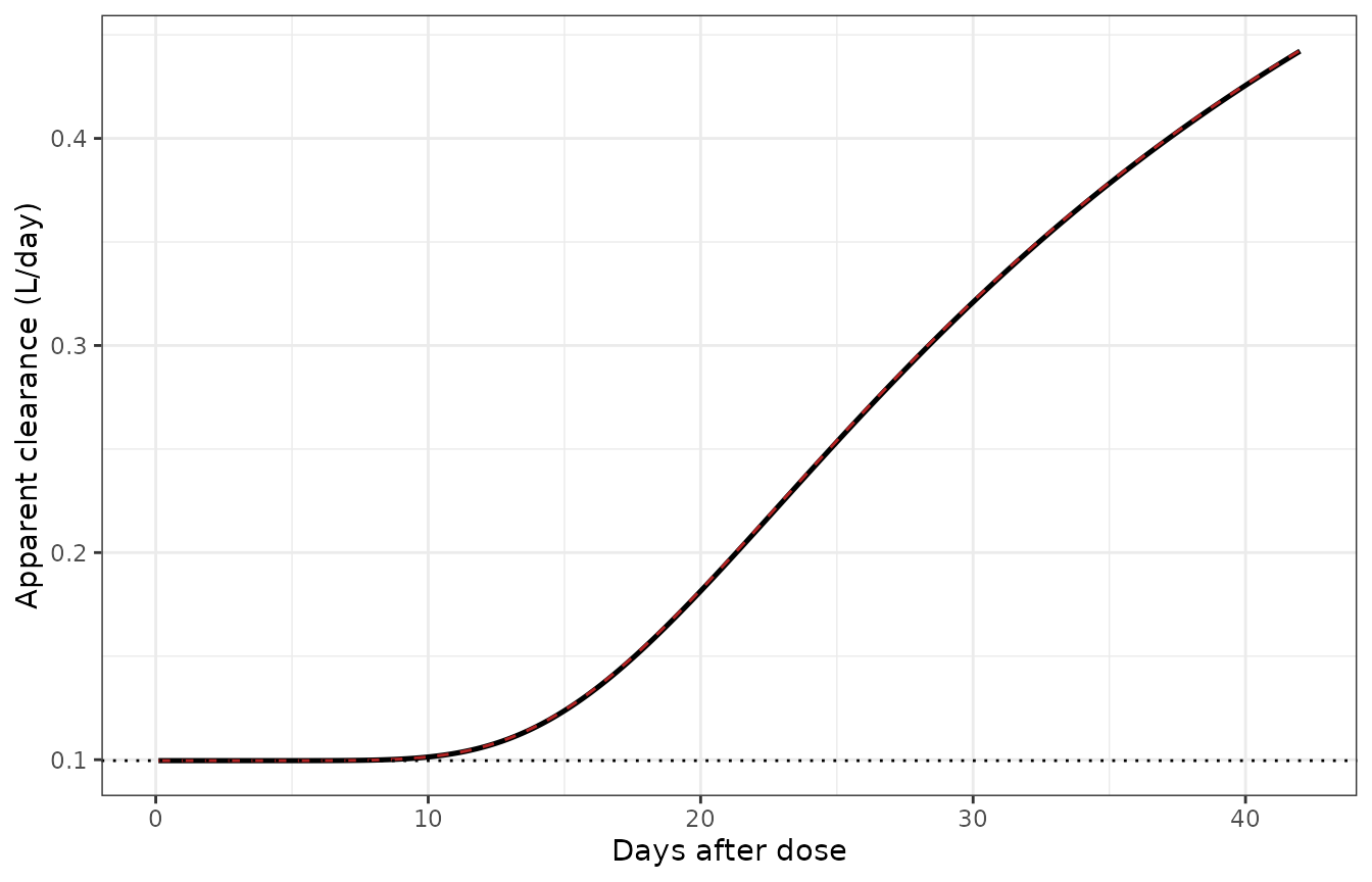
Apparent clearance over 42 days for the typical child at BSA 0.79 m^2, with the closed-form prediction overlaid. Model-derived; not a published figure.
c(start = min(ramp$cl_app),
  day14 = ramp$cl_app[which.min(abs(ramp$time - 14))],
  day42 = max(ramp$cl_app),
  max_pct_diff_vs_closed_form = max(abs(100 * (ramp$cl_app - ramp$cl_cf) / ramp$cl_cf)))
#>                       start                       day14
#>                   0.0995400                   0.1161685
#>                       day42 max_pct_diff_vs_closed_form
#>                   0.4421449                   0.3313770

# The solve and its own closed form use the same parameters, so the difference
# is pure numerical error and a tight bound is correct.
stopifnot(
  abs(min(ramp$cl_app) - CL0) / CL0 < 0.01,
  all(diff(ramp$cl_app) > -1e-9),
  max(ramp$cl_app) < CL0 + Q0,
  max(abs((ramp$cl_app - ramp$cl_cf) / ramp$cl_cf)) < 0.01
)
Mass balance
For this linear chain, with ke = CLinitial / V,
kt = Qtr / V and ratio = kt / (ke + kt), the
total AUC of a dose D is
D / (V * (ke + kt)) * sum(ratio^j, j = 0..13). Reproducing
it from the solved ODEs confirms that the chain is wired correctly and
conserves mass.
ev_mb <- rxode2::et(amt = 2500 * 0.79, cmt = "central") |>
  rxode2::et(seq(0, 150, by = 0.01), cmt = "central") |>
  as.data.frame() |>
  mutate(BSA = 0.79, AGE = 5, SEXF = 0, OCC = 1)
mb <- rxode2::rxSolve(mod0, ev_mb, returnType = "data.frame")
#> ℹ omega/sigma items treated as zero: 'etalcl', 'etaiov_vc_1', 'etaiov_vc_2', 'etaiov_vc_3', 'etaiov_cl_1', 'etaiov_cl_2', 'etaiov_cl_3'

auc_num <- sum(diff(mb$time) * (head(mb$Cc, -1) + tail(mb$Cc, -1)) / 2)
ke <- CL0 / V0
kt <- Q0 / V0
r <- kt / (ke + kt)
auc_cf <- 2500 * 0.79 / (V0 * (ke + kt)) * sum(r^(0:13))

c(numeric = auc_num, closed_form = auc_cf, pct_diff = 100 * (auc_num - auc_cf) / auc_cf)
#>      numeric  closed_form     pct_diff
#> 1.656364e+04 1.656364e+04 5.548814e-06
stopifnot(abs(auc_num - auc_cf) / auc_cf < 0.005)
How the printed values are quoted
Table 3 prints V, CLinitial and
Qtr in L/m^2 and L/day/m^2, but
the control stream multiplies nothing by BSA: the whole BSA dependence
is the linear centred term
THETA * (1 + F_BSA * (BSA - 0.79)), so each THETA is an
absolute value for a child at the 0.79 m^2 centring point. The Table 3
footnote states how the printed numbers were obtained from those
THETAs:
During NONMEM estimation, values for CLinitial, CLinduced, Qtr and V are reported for BSA=0.79 m2; values were converted from L/day/0.79m2 or L/0.79m2 to L/day/m2 or L/m2 for better comparison.
That is a division by 0.79, so the model multiplies each printed
value by 0.79 m^2 to recover the THETA. The later papers from the same
group (Siebel 2022 and Wurthwein 2025) describe the same convention as
quoting values “for a child with BSA = 1 m^2”, which read literally
would instead mean THETA = printed / (1 + F_BSA * 0.21).
The two readings differ by 4.9% on V and 2.9% on
CLinitial and Qtr. This model follows the
arithmetic stated in this paper’s own footnote. The table below shows
what that choice changes.
tibble::tibble(
  Parameter = c("V", "CLinitial", "Qtr"),
  Printed = c(1.69, 0.126, 0.918),
  `THETA, printed x 0.79 (used)` = c(1.69, 0.126, 0.918) * 0.79,
  `THETA, printed at BSA = 1 m^2` = c(1.69 / (1 + 1.56 * 0.21),
                                      0.126 / (1 + 1.44 * 0.21),
                                      0.918 / (1 + 1.44 * 0.21))
) |>
  mutate(`Difference (%)` = 100 * (`THETA, printed x 0.79 (used)` /
                                     `THETA, printed at BSA = 1 m^2` - 1)) |>
  knitr::kable(digits = c(0, 3, 4, 4, 1), caption = paste(
    "Printed values are per m^2 (L/m^2, L/day/m^2); the THETAs are absolute",
"values (L, L/day) for a child at BSA 0.79 m^2."))| Parameter | Printed | THETA, printed x 0.79 (used) | THETA, printed at BSA = 1 m^2 | Difference (%) |
|---|---|---|---|---|
| V | 1.690 | 1.3351 | 1.2730 | 4.9 |
| CLinitial | 0.126 | 0.0995 | 0.0967 | 2.9 |
| Qtr | 0.918 | 0.7252 | 0.7049 | 2.9 |
Neither the published activity medians nor the external evidence separates the two readings. The typical-value checks in the next section land within 5% of the observed medians either way. The Discussion’s statement that the re-induction volume has a median of 44.4 mL/kg is somewhat closer to the BSA = 1 m^2 reading (about 46 mL/kg for the median child of Table 1, against about 48 mL/kg with the reading used here). That statistic is a median over individual Bayesian estimates, though, and the weight distribution needed to reproduce it is not published.
# Re-induction volume of the Table 1 median child (BSA 0.78 m^2, 19.55 kg),
# under each reading, in mL/kg. The published value is 44.4 mL/kg.
f_v <- (1 + 1.56 * (0.78 - 0.79)) * (1 - 0.284)
c(printed_x_0.79 = 1000 * 1.69 * 0.79 * f_v / 19.55,
  bsa_1m2 = 1000 * 1.69 / (1 + 1.56 * 0.21) * f_v / 19.55)
#> printed_x_0.79        bsa_1m2
#>       48.13397       45.89415
Source trace
Every ini() entry carries an in-file comment naming its
source.
| Item | Value(s) | Source location |
|---|---|---|
| Chain of 14 serial compartments; dose into compartment 1 | topology | Figure 1; ESM Section 4 $MODEL / $DES
|
Terminal compartment loses CLinitial + Qtr
(CLinduced = Qtr) |
structural | Figure 1 caption; Table 3 footnote (a); ESM Section 2 |
Observation = total activity over all 14 states divided by
V
|
structural | ESM Section 4 $ERROR
(TOT = A(1)+...+A(14); IPRED = TOT/V1) |
BSA linear and centred on 0.79 m^2; one slope on V, one
shared by CLinitial and Qtr
|
form + constant | Table 3 footnote (b); ESM Section 4 $PK
(SCV1, SCCL) |
Printed V, CLinitial, Qtr =
THETA / 0.79 |
conversion | Table 3 footnote |
| Age hockey stick, break point fixed at 8 years | form + constant | Table 3 footnote (d); ESM Section 4 $PK
(THETA(13) = 0 FIX); ESM Section 2 |
Sex effect on CLinitial, males the reference |
form | Table 3 footnote (e); ESM Section 4 $PK
(SEX.EQ.1 = 1) |
Phase effects as (1 + F) against the first induction
dose |
form | Table 3 footnote (c); ESM Section 4 $PK
(V1KOV, CLKOV) |
IIV on CLinitial only; IIV on V and
Qtr fixed to 0 |
structure | ESM Section 4 $OMEGA; ESM Section 2 |
IOV on V and CLinitial, one variance per
parameter shared across occasions |
structure | ESM Section 4 $OMEGA BLOCK(1) SAME
|
| Combined proportional + additive residual SD | form | ESM Section 4 $ERROR + $SIGMA 1 FIX
|
V 1.69, CLinitial 0.126, Qtr
0.918 |
per m^2 | Table 3, Final PK model |
F_BSA on V 1.56; on
CLinitial + Qtr 1.44 |
slopes | Table 3, Final PK model |
Phase changes -0.159, -0.284 (V); -0.110, -0.412
(CLinitial) |
fractions | Table 3, Final PK model |
| Age > 8 years 0.018; sex -0.071 | slope, fraction | Table 3, Final PK model |
IIV CLinitial 24.0%; IOV V 13.3%; IOV
CLinitial 22.4% |
CV | Table 3, Final PK model |
| Proportional 18.9%; additive 8.74 U/L | SD | Table 3, Final PK model |
| Dose-normalized activity percentiles used below | U/L | Table 2 |
Reproducing the published activity levels
Table 2 reports percentiles of asparaginase activity 7 and 14 days
after each administration, normalized to a 2500 U/m^2 dose. A
typical-value solve at 2500 U/m^2 is compared with the medians. The
model has males as the reference for CLinitial, so male and
female solves are averaged with the pooled Table 1 weights (1520 male,
1107 female).
The day-14 sample after the first induction dose falls on the day of
the second dose. Because V switches stepwise at the new
occasion, the value is read just before the switch.
# OCC steps at each administration. It is a time-varying covariate, so it is
# attached to a materialized data frame (assignments onto an rxEt object are
# silently dropped).
run_series <- function(m, dose_times, occs, bsa, age, sexf, tail_days = 16,
                       by = 0.05) {
  grid <- seq(0, max(dose_times) + tail_days, by = by)
  ev <- rxode2::et(amt = 2500 * bsa, time = dose_times, dur = 2 / 24,
                   cmt = "central") |>
    rxode2::et(grid, cmt = "central") |>
    as.data.frame()
  idx <- findInterval(ev$time, dose_times)
  idx[idx < 1] <- 1
  ev$OCC <- occs[idx]
  ev$BSA <- bsa
  ev$AGE <- age
  ev$SEXF <- sexf
  rxode2::rxSolve(m, ev, returnType = "data.frame")
}

# Last grid point strictly before `tt` (pre-switch when `tt` is a dose time).
at_day <- function(sim, tt) sim$Cc[max(which(sim$time < tt - 1e-9))]

typical_levels <- function(sexf) {
  ind <- run_series(mod0, c(0, 14), c(1, 2), bsa = 0.78, age = 5.13, sexf = sexf)
  rei <- run_series(mod0, 0, 3, bsa = 0.78, age = 5.13, sexf = sexf)
  c(at_day(ind, 7), at_day(ind, 14), at_day(ind, 21), at_day(ind, 28),
    at_day(rei, 7), at_day(rei, 14))
}
w_female <- 1107 / (1520 + 1107)
sim_typ <- (1 - w_female) * typical_levels(0) + w_female * typical_levels(1)
#> ℹ omega/sigma items treated as zero: 'etalcl', 'etaiov_vc_1', 'etaiov_vc_2', 'etaiov_vc_3', 'etaiov_cl_1', 'etaiov_cl_2', 'etaiov_cl_3'
#> ℹ omega/sigma items treated as zero: 'etalcl', 'etaiov_vc_1', 'etaiov_vc_2', 'etaiov_vc_3', 'etaiov_cl_1', 'etaiov_cl_2', 'etaiov_cl_3'
#> ℹ omega/sigma items treated as zero: 'etalcl', 'etaiov_vc_1', 'etaiov_vc_2', 'etaiov_vc_3', 'etaiov_cl_1', 'etaiov_cl_2', 'etaiov_cl_3'
#> ℹ omega/sigma items treated as zero: 'etalcl', 'etaiov_vc_1', 'etaiov_vc_2', 'etaiov_vc_3', 'etaiov_cl_1', 'etaiov_cl_2', 'etaiov_cl_3'

tab2 <- tibble::tibble(
  Administration = rep(c("Induction 1st", "Induction 2nd", "Reinduction"), each = 2),
  Day = rep(c(7, 14), 3),
  Simulated = sim_typ,
  Published = c(896, 543, 1259, 629, 1437, 751)
) |>
  mutate(`Difference (%)` = 100 * (Simulated - Published) / Published)

knitr::kable(tab2, digits = c(0, 0, 0, 0, 1),
caption = "Typical-value activity (U/L) versus the Table 2 medians.")| Administration | Day | Simulated | Published | Difference (%) |
|---|---|---|---|---|
| Induction 1st | 7 | 900 | 896 | 0.4 |
| Induction 1st | 14 | 530 | 543 | -2.4 |
| Induction 2nd | 7 | 1293 | 1259 | 2.7 |
| Induction 2nd | 14 | 614 | 629 | -2.4 |
| Reinduction | 7 | 1373 | 1437 | -4.5 |
| Reinduction | 14 | 743 | 751 | -1.0 |
# A mis-transcribed volume, clearance, dose or unit moves every row by tens of
# percent. These are deterministic solves, so the bounds are stable.
stopifnot(
  abs(median(tab2$`Difference (%)`)) < 5,
  max(abs(tab2$`Difference (%)`)) < 10
)
All six typical-value levels are within 5% of the published medians, and five of the six fall below them. In the stochastic comparison further down, the largest shortfall is day 14 after the second induction dose. The authors report the same for their own model: the pcVPC slightly underpredicts day-14 levels after the second induction dose (Section 3.2.3), and external validation showed a bias of -5.5% for day 14 in induction (Section 3.2.4).
Virtual cohort
Only the median and range of BSA and age are published (Table 1), so the cohort uses log-normal distributions matched to the model-building medians and truncated to the published ranges. It is sampled on a deterministic quantile lattice, which makes it identical on every machine. BSA and age share a lattice position because both are driven by growth.
n_sub <- 200L
p <- (seq_len(n_sub) - 0.5) / n_sub

cohort <- tibble::tibble(
  id   = seq_len(n_sub),
  BSA  = pmin(pmax(qlnorm(p, log(0.78), 0.38), 0.41), 2.42),
  AGE  = pmin(pmax(qlnorm(p, log(5.13), 0.50), 1.03), 17.9),
  # 42.1% female, assigned by a Weyl sequence so the marginal is exact without
  # correlating sex with the BSA / age lattice position.
  SEXF = as.integer(((seq_len(n_sub) * 0.421) %% 1) < 0.421)
) |>
  # 2500 U/m^2 with the protocol cap of 3750 U per dose.
  mutate(amt = pmin(2500 * BSA, 3750))

summarise(cohort, bsa_median = median(BSA), age_median = median(AGE),
          pct_female = 100 * mean(SEXF))
#> # A tibble: 1 × 3
#>   bsa_median age_median pct_female
#>        <dbl>      <dbl>      <dbl>
#> 1 0.780 5.13 42Stochastic simulation
A stochastic run exercises the IIV on CLinitial (24.0%)
and the IOV on CLinitial (22.4%) and V
(13.3%). Table 2 reports the observed 25th, 50th and 75th percentiles,
normalized to 2500 U/m^2, so the simulated values are dose-normalized
the same way before comparison. Residual error is not added: the
comparison is of the concentration distribution.
pop_events <- function(dose_times, occs, obs) {
  lapply(cohort$id, function(i) {
    ci <- cohort[cohort$id == i, ]
    e <- rxode2::et(amt = ci$amt, time = dose_times, dur = 2 / 24,
                    cmt = "central") |>
      rxode2::et(obs, cmt = "central") |>
      as.data.frame()
    e$id <- i
    e
  }) |>
    dplyr::bind_rows() |>
    mutate(OCC = occs[pmax(findInterval(time, dose_times), 1)]) |>
    left_join(select(cohort, id, BSA, AGE, SEXF), by = "id")
}

obs_ind <- sort(unique(c(seq(0, 28, by = 0.25), 13.99)))
ind_pop <- rxode2::rxSolve(mod, pop_events(c(0, 14), c(1, 2), obs_ind),
                           returnType = "data.frame")
rei_pop <- rxode2::rxSolve(mod, pop_events(0, 3, seq(0, 14, by = 0.25)),
                           returnType = "data.frame")

# Dose-normalize to 2500 U/m^2 as in Table 2.
norm <- function(sim) {
  left_join(sim, select(cohort, id, bsa_i = BSA, dose_i = amt), by = "id") |>
    mutate(Cn = Cc * 2500 * bsa_i / dose_i)
}
ind_pop <- norm(ind_pop)
rei_pop <- norm(rei_pop)

pick <- function(sim, tt) sim$Cn[abs(sim$time - tt) < 1e-6]
q3 <- function(x) quantile(x, c(0.25, 0.5, 0.75), names = FALSE)

vpc_tab <- tibble::tibble(
  Administration = rep(c("Induction 1st", "Induction 2nd", "Reinduction"), each = 2),
  Day = rep(c(7, 14), 3),
  sim = list(q3(pick(ind_pop, 7)), q3(pick(ind_pop, 13.99)),
             q3(pick(ind_pop, 21)), q3(pick(ind_pop, 28)),
             q3(pick(rei_pop, 7)), q3(pick(rei_pop, 14))),
  pub = list(c(737, 896, 1076), c(428, 543, 662), c(991, 1259, 1623),
             c(473, 629, 782), c(1205, 1437, 1722), c(618, 751, 883))
) |>
  mutate(
    `Sim P25` = sapply(sim, `[`, 1), `Sim P50` = sapply(sim, `[`, 2),
    `Sim P75` = sapply(sim, `[`, 3),
    `Obs P25` = sapply(pub, `[`, 1), `Obs P50` = sapply(pub, `[`, 2),
    `Obs P75` = sapply(pub, `[`, 3),
    `Median diff (%)` = 100 * (`Sim P50` - `Obs P50`) / `Obs P50`
  ) |>
  select(-sim, -pub)

knitr::kable(vpc_tab, digits = 0,
             caption = paste("Simulated (200 virtual patients) versus observed",
"Table 2 percentiles of dose-normalized activity (U/L)."))| Administration | Day | Sim P25 | Sim P50 | Sim P75 | Obs P25 | Obs P50 | Obs P75 | Median diff (%) |
|---|---|---|---|---|---|---|---|---|
| Induction 1st | 7 | 783 | 881 | 983 | 737 | 896 | 1076 | -2 |
| Induction 1st | 14 | 406 | 514 | 604 | 428 | 543 | 662 | -5 |
| Induction 2nd | 7 | 1084 | 1263 | 1467 | 991 | 1259 | 1623 | 0 |
| Induction 2nd | 14 | 448 | 588 | 756 | 473 | 629 | 782 | -7 |
| Reinduction | 7 | 1228 | 1380 | 1532 | 1205 | 1437 | 1722 | -4 |
| Reinduction | 14 | 588 | 714 | 866 | 618 | 751 | 883 | -5 |
# Assert on the centre of the cohort, not its tails: the extremes of a random
# cohort are not reproducible across rxode2 builds.
stopifnot(
  n_distinct(ind_pop$id) == n_sub, !anyNA(ind_pop$Cc), !anyNA(rei_pop$Cc),
  abs(median(vpc_tab$`Median diff (%)`)) < 10,
  quantile(abs(vpc_tab$`Median diff (%)`), 0.9) < 20,
  # The variability must be doing something: a simulated interquartile range
  # of at least half the observed one at every time point.
  all((vpc_tab$`Sim P75` - vpc_tab$`Sim P25`) >
        0.5 * (vpc_tab$`Obs P75` - vpc_tab$`Obs P25`))
)
qs <- ind_pop |>
  group_by(time) |>
  summarise(lo = quantile(Cn, 0.25), md = median(Cn), hi = quantile(Cn, 0.75),
            .groups = "drop")
obs_pts <- tibble::tibble(
  time = c(7, 14, 21, 28),
  md = c(896, 543, 1259, 629),
  lo = c(737, 428, 991, 473),
  hi = c(1076, 662, 1623, 782)
)

ggplot(qs, aes(time)) +
  geom_ribbon(aes(ymin = lo, ymax = hi), alpha = 0.2) +
  geom_line(aes(y = md), linewidth = 0.8) +
  geom_pointrange(data = obs_pts, aes(y = md, ymin = lo, ymax = hi),
                  colour = "firebrick") +
  labs(x = "Days from the first induction dose",
       y = "Asparaginase activity (U/L)") +
  theme_bw()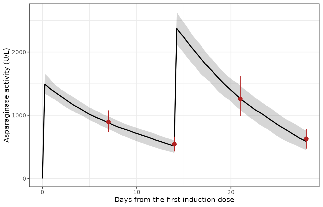
Simulated induction profiles for 200 virtual patients (median and 25th-75th percentile band, dose-normalized to 2500 U/m^2) with the Table 2 observed quartiles overlaid. Compare Figure 3 of Wurthwein 2021.
PKNCA validation
PKNCA computes exposure over the first induction dosing interval (one
dose, occasion 1, 0-14 days) for a typical-value version of the cohort,
grouped by BSA band. The concentration frame is filtered only on
!is.na(Cc), which keeps the time-zero record.
pk_cohort <- cohort[seq(1, n_sub, by = 2), ] |>
  mutate(treatment = factor(
    case_when(BSA < 0.6 ~ "Low (<0.6 m^2)",
              BSA < 1.1 ~ "Mid (0.6-1.1 m^2)",
              TRUE      ~ "High (>=1.1 m^2)"),
    levels = c("Low (<0.6 m^2)", "Mid (0.6-1.1 m^2)", "High (>=1.1 m^2)")))

grid_nca <- sort(unique(c(seq(0, 14, by = 0.25), seq(0, 1, by = 0.05))))
ev_nca <- lapply(pk_cohort$id, function(i) {
  ci <- pk_cohort[pk_cohort$id == i, ]
  e <- rxode2::et(amt = ci$amt, dur = 2 / 24, cmt = "central") |>
    rxode2::et(grid_nca, cmt = "central") |>
    as.data.frame()
  e$id <- i
  e
}) |>
  dplyr::bind_rows() |>
  mutate(OCC = 1) |>
  left_join(select(pk_cohort, id, BSA, AGE, SEXF), by = "id")

sim_nca <- rxode2::rxSolve(mod0, ev_nca, returnType = "data.frame")
#> ℹ omega/sigma items treated as zero: 'etalcl', 'etaiov_vc_1', 'etaiov_vc_2', 'etaiov_vc_3', 'etaiov_cl_1', 'etaiov_cl_2', 'etaiov_cl_3'
#> Warning: multi-subject simulation without without 'omega'

nca_conc <- sim_nca |>
  filter(!is.na(Cc)) |>
  left_join(select(pk_cohort, id, treatment), by = "id") |>
  select(id, time, Cc, treatment)
nca_dose <- pk_cohort |>
  transmute(id, time = 0, amt, treatment)

conc_obj <- PKNCA::PKNCAconc(nca_conc, Cc ~ time | treatment + id,
                             concu = "U/L", timeu = "day")
dose_obj <- PKNCA::PKNCAdose(nca_dose, amt ~ time | treatment + id, doseu = "U")
intervals <- data.frame(start = 0, end = 14, cmax = TRUE, tmax = TRUE,
                        auclast = TRUE, half.life = TRUE)
nca_res <- PKNCA::pk.nca(PKNCA::PKNCAdata(conc_obj, dose_obj, intervals = intervals))

as.data.frame(nca_res) |>
  filter(PPTESTCD %in% c("cmax", "tmax", "auclast", "half.life")) |>
  group_by(treatment, PPTESTCD) |>
  summarise(median = median(PPORRES, na.rm = TRUE), .groups = "drop") |>
  tidyr::pivot_wider(names_from = PPTESTCD, values_from = median) |>
  dplyr::rename(
    "BSA band"           = treatment,
    "AUC0-14d (U*day/L)" = auclast,
    "Cmax (U/L)"         = cmax,
    "t1/2 (day)"         = "half.life",
    "Tmax (day)"         = tmax
  ) |>
knitr::kable(digits = 2, caption = "PKNCA medians per BSA band, first induction dose.")| BSA band | AUC0-14d (U*day/L) | Cmax (U/L) | t1/2 (day) | Tmax (day) |
|---|---|---|---|---|
| Low (<0.6 m^2) | 14597.75 | 1699.77 | 7.50 | 0.1 |
| Mid (0.6-1.1 m^2) | 12912.95 | 1467.17 | 9.19 | 0.1 |
| High (>=1.1 m^2) | 11902.14 | 1351.45 | 9.40 | 0.1 |
Comparison against closed-form expectations
The paper publishes no NCA table, so the reference is a closed form
of the published parameters. Over a 0-14-day window the decline is
governed by CLinitial with slight curvature, so the
relevant reference is the initial-phase half-life
ln(2) * V / CLinitial, computed per subject from that
subject’s covariates. The NCA value must sit just below it because
apparent clearance is already rising. The asymptotic half-life
ln(2) * V / (CLinitial + Qtr) (about 1.1 days) is never
reached in the window and is not a valid reference.
ref_hl <- pk_cohort |>
  mutate(
    v_i  = 1.69 * 0.79 * (1 + 1.56 * (BSA - 0.79)),
    cl_i = 0.126 * 0.79 * (1 + 1.44 * (BSA - 0.79)) *
      (1 + 0.018 * (AGE - 8) * (AGE > 8)) * (1 - 0.071 * SEXF),
    hl_ref = log(2) * v_i / cl_i
  )

reference <- ref_hl |>
  group_by(treatment) |>
  summarise(PPORRES = median(hl_ref), .groups = "drop") |>
  mutate(PPTESTCD = "half.life")

cmp <- nlmixr2lib::ncaComparisonTable(
  simulated     = nca_res,
  reference     = reference,
  by            = "treatment",
  units         = c(half.life = "day"),
  tolerance_pct = 20
)
knitr::kable(cmp, caption = paste(
  "NCA half-life over 0-14 days versus the per-subject initial-phase closed",
"form, median per BSA band. * marks rows differing by >20%."))| NCA parameter | treatment | Reference | Simulated | % diff |
|---|---|---|---|---|
| t½ (day) | Low (<0.6 m^2) | 8.97 | 7.5 | -16.3% |
| t½ (day) | Mid (0.6-1.1 m^2) | 9.48 | 9.19 | -3.0% |
| t½ (day) | High (>=1.1 m^2) | 9.49 | 9.4 | -0.9% |
hl_band <- as.data.frame(nca_res) |>
  filter(PPTESTCD == "half.life") |>
  group_by(treatment) |>
  summarise(nca = median(PPORRES, na.rm = TRUE), .groups = "drop") |>
  left_join(dplyr::rename(reference, ref = PPORRES), by = "treatment") |>
  mutate(pct = 100 * (nca - ref) / ref)
as.data.frame(hl_band)
#>           treatment      nca      ref  PPTESTCD         pct
#> 1    Low (<0.6 m^2) 7.503002 8.969116 half.life -16.3462504
#> 2 Mid (0.6-1.1 m^2) 9.189223 9.476167 half.life  -3.0280593
#> 3  High (>=1.1 m^2) 9.402529 9.485026 half.life  -0.8697595

hl_asympt <- log(2) * V0 / (CL0 + Q0)
stopifnot(
  all(hl_band$nca < hl_band$ref),
  all(hl_band$nca > 3 * hl_asympt),
  max(abs(hl_band$pct)) < 20
)
Errata
No discrepancy affecting a model value was found. Two points of presentation:
-
Table 3 layout. In the typeset table the
CLinducedrow of the structural-model column (0.740) sits on the same line asCLinitial, and the covariate labels are split across lines. The values were read from the column layout and cross-checked against the bootstrap column and the percentages in the Abstract and Section 4.1 (for example -41.2% and -28.4% for re-induction match -0.412 and -0.284). -
The ESM Section 4
$THETAblock lists initial estimates, not final ones (for exampleTHETA(1)= 1.25,$OMEGAIIVCLP= 0.0567). All final values are taken from Table 3; the control stream is used only for the model structure and the fixed constants.
Assumptions and deviations
-
Printed
V,CLinitialandQtrare multiplied by 0.79 m^2. This follows the Table 3 footnote. The alternative reading used by the same group’s later papers would lower these three values by 2.9-4.9%; see “How the printed values are quoted” above. - BSA centring constant 0.79 m^2 is taken from the control stream and Table 3 footnote (b). It is the Structural Model Dataset median; the model-building median in Table 1 is 0.78 m^2.
-
Compartment naming. The control stream names the
states
CENTRALandPERI2-PERI14. They are not classical peripheral compartments (there is no back-flow, and all share one volume), so thetransit<n>prefix is used, withcentralkept for the dosed compartment. -
OCCcarries both the phase effect and the IOV, as in the authors’ control stream. The occasion codes2/3/5are renumbered to1/2/3. -
$OMEGA BLOCK(1) SAMEhas no nlmixr2 equivalent. Occasions 2 and 3 carry their own eta, with the variance fixed to the occasion-1 estimate. -
IIV and IOV percentages are taken as log-normal
CVs,
omega^2 = log(1 + CV^2), because the variability is exponential in the control stream. - Cohort distributions are assumed. Log-normal BSA and age matched to the Table 1 medians and ranges, on a shared deterministic lattice. The same cohort is used for the re-induction dose, although in the trial only non-high-risk patients received it, about 4 months later.
-
Concentration is discontinuous at an occasion
switch because
Vchanges stepwise between administrations. NONMEM behaves the same way. Troughs at a dose time are read just before the switch. - Silent inactivation and hypersensitivity are out of scope. Do not use the model to predict activity in an inactivating patient.
Reference
Wurthwein G, Lanvers-Kaminsky C, Siebel C, et al. Population Pharmacokinetics of PEGylated Asparaginase in Children with Acute Lymphoblastic Leukemia: Treatment Phase Dependency and Predictivity in Case of Missing Data. Eur J Drug Metab Pharmacokinet. 2021;46(2):289-300. https://doi.org/10.1007/s13318-021-00670-8