Levonorgestrel (Adeojo 2024)
Source:vignettes/articles/Adeojo_2024_levonorgestrel.Rmd
Adeojo_2024_levonorgestrel.RmdModel and source
- Citation: Adeojo LW, Patel RC, Sambol NC. A Physiologically-Based Pharmacokinetic Simulation to Evaluate Approaches to Mitigate Efavirenz-Induced Decrease in Levonorgestrel Exposure with a Contraceptive Implant. Pharmaceutics. 2024;16(8):1050. doi:10.3390/pharmaceutics16081050. Parameter estimates from Supplementary Table S2; study designs from Supplementary Table S1.
- Description: MBMA. Two-compartment population PK model for levonorgestrel fit to pooled MEAN plasma concentration-time profiles digitised from four published trials (Adeojo 2024). The four trials span single 0.25 mg oral, single 0.25 mg intravenous, single 0.75 mg oral, two-dose 0.75 mg oral, and 150 mg subdermal implant administration in women, with two of the trials contributing arms co-administered with efavirenz 600 mg orally once daily. Absorption is first-order and applies to oral dosing only (ka fixed at 4.15 /h); the intravenous and subdermal-implant routes enter the central compartment directly, so the estimated bioavailability F is an oral bioavailability. Concomitant efavirenz enters as a single binary covariate with two effects: clearance rises from 5.86 to 10.1 L/h (+72.4%) through CYP3A4 induction and oral bioavailability falls from 0.837 to 0.533 (-36.3%) through gut-wall CYP3A4 induction. The model carries BETWEEN-STUDY variability on oral bioavailability only (21.2% CV) and no between-subject variability, because it was fit to study-level mean profiles rather than individual concentrations; it therefore simulates study-level mean concentration-time curves, NOT individual patient concentrations. This is the reference mixed-effects model of the source paper, used there to anchor a Simcyp physiologically-based model by retrograde determination; the Simcyp PBPK model itself is not reproducible from the published sources and is not packaged here (see the validation vignette Assumptions and deviations).
- Article: https://doi.org/10.3390/pharmaceutics16081050
- Supplement (Tables S1 and S2): https://www.mdpi.com/article/10.3390/pharmaceutics16081050/s1
What this paper contains, and what is packaged here
Adeojo 2024 reports two models:
- A mixed-effects model (MEM) built in NONMEM 7.4.2
from pooled mean levonorgestrel concentration-time profiles
digitised from four published trials. This is the model packaged as
Adeojo_2024_levonorgestrel. Its parameters are fully reported in Supplementary Table S2, and its clearance and bioavailability estimates, with and without efavirenz, are the paper’s reference values. - A Simcyp physiologically-based (PBPK) model for levonorgestrel, built with the Simcyp v19.1 “minimum PKPD” option and combined with the efavirenz induction model already shipped inside Simcyp. This model is not packaged, because it is not reproducible from any published source: the paper reports only the eight levonorgestrel-specific drug inputs of its Table 1, while the whole-body physiology (organ volumes, blood flows, CYP3A4 abundance for the simulated population, gut model) and the entire efavirenz induction parameterisation are Simcyp platform content that is never written out as equations or values. Filling those in from class knowledge would be unauditable, so it is deliberately omitted rather than approximated. See “Assumptions and deviations”.
The two models are tightly coupled in the source: the PBPK model’s unknown intrinsic clearance terms were set by retrograde determination so that the PBPK model would reproduce the MEM’s clearance values. That coupling is what makes the checks in this vignette possible - several numbers the paper attributes to the PBPK model can be recovered exactly from the packaged MEM.
Population
The model was fit to aggregate data pooled across four trials in adult women (Adeojo 2024 Supplementary Table S1), 80 distinct participants in total:
- Back 1987 (n = 5): levonorgestrel 0.25 mg orally and 0.25 mg intravenously in a crossover, co-administered with ethinylestradiol. The intravenous arm is what makes absolute oral bioavailability identifiable.
- Kook 2002 (n = 16): levonorgestrel 0.75 mg single oral dose.
- Carten 2012 (n = 21): levonorgestrel 0.75 mg x 2 orally, doses 12 h apart, PK sampling from 12 h, in a crossover with and without efavirenz.
- Scarsi 2016 (n = 18 without efavirenz, n = 20 with efavirenz): levonorgestrel 150 mg subdermal implant (two rods), plasma concentrations over 48 weeks, in women living with HIV.
Every efavirenz-exposed arm used efavirenz 600 mg orally once daily.
The observations were mean concentration among subjects at each nominal time point, read off the published figures with GraphClick 3.0; individual concentration-time data were not available to the authors (Adeojo 2024 Section 2.2). Two levels of random effects were recognised: between-study variability of bioavailability, and within-study variability of the mean concentrations. The limited number of studies did not permit estimating between-study variability on any other parameter. This is therefore a meta-analytic fit that simulates study-level mean profiles, not individual patient concentrations.
The same information is available programmatically via
readModelDb("Adeojo_2024_levonorgestrel")()$population.
Source trace
Every ini() entry carries an in-file comment naming its
source location in
inst/modeldb/specificDrugs/Adeojo_2024_levonorgestrel.R.
They are collected here for review.
| Equation / parameter | Value | Source location |
|---|---|---|
lka |
log(4.15) /h |
Supp Table S2 row ka; footnote * marks it
fixed, not estimated |
lcl |
log(5.86) L/h |
Supp Table S2 row CL (95% CI 4.97, 6.75) |
lvc |
log(49.5) L |
Supp Table S2 row Vcentral (95% CI 36.3, 62.7) |
lq |
log(10.2) L/h |
Supp Table S2 row Q (95% CI 6.9, 13.5); also main Table
1 row Q (L/h), source MEM
|
lvp |
log(105) L |
Supp Table S2 row Vperipheral (95% CI 85.6, 124.4) |
lfdepot |
log(0.837) |
Supp Table S2 row Foral (95% CI 0.736, 0.938) |
e_conmed_efv_cl |
0.7235 |
Derived: (10.1 - 5.86) / 5.86, from Supp Table S2 rows
CL and CLwith efavirenz (10.1 L/h, 95% CI
9.09, 11.1) |
e_conmed_efv_fdepot |
-0.3632 |
Derived: (0.533 - 0.837) / 0.837, from Supp Table S2
rows Foral and Foral, with efavirenz (0.533,
95% CI 0.427, 0.639) |
eta_study_lfdepot |
0.043963 |
Supp Table S2 Foral inter-study variability 21.2% (95%
CI 0, 30.1); omega^2 = log(1 + 0.212^2)
|
addSd |
0.214 ng/mL |
Supp Table S2
Intra-study variability in mean concentrations, additive
component (95% CI 0.157, 0.258) |
propSd |
0.084 |
Supp Table S2 same block, proportional component 8.4% (95% CI 0, 12.2) |
| Two-compartment disposition with first-order oral absorption | n/a | Section 2.2: “The model employed a two-compartment model, with first-order absorption for oral dosing only” |
Implant release rates (used to build the event table below, not an
ini() parameter) |
100, 89, 73, 40, 35, 30 ug/day at months 1, 3, 6, 12, 24, 36 | Table 1 row Release rate, source reference [8];
footnote a states these are amounts reaching systemic
circulation, footnote b marks the interpolated
entries. The ~25 ug/day at 5 years is from the Introduction and the
Table 1 key. |
| Reference values used for validation below | CL 5.86 and 10.10 L/h; CL/F 7.00 and 18.95 L/h; implant 284, 213, 177 pg/mL at 1, 3, 5 years | Results, paragraphs 1 and 2 |
mod <- readModelDb("Adeojo_2024_levonorgestrel")Oral and intravenous arms
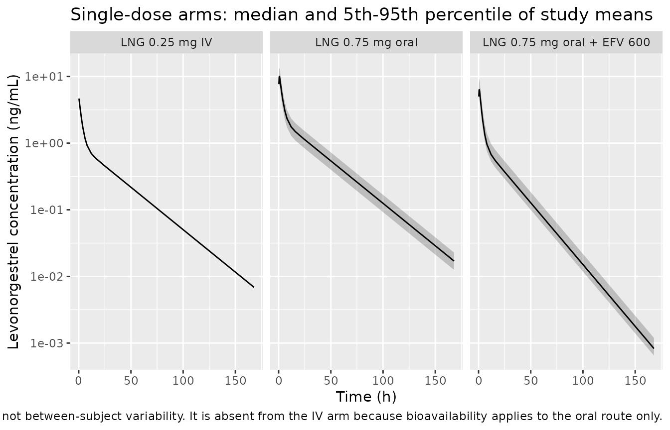
Three single-dose arms reproduce the routes that identify the model’s clearance and bioavailability terms: 0.75 mg orally with and without efavirenz, and 0.25 mg intravenously.
set.seed(20240807)

obs_times <- c(0, 0.25, 0.5, 0.75, 1, 1.5, 2, 3, 4, 6, 8, 12, 16, 24,
               36, 48, 72, 96, 120, 144, 168)

# `cmt` on observation rows is always an ODE STATE name ("central"), never the
# algebraic observable name ("Cc"). rxode2 returns Cc as a column regardless.
make_arm <- function(n, label, amt, cmt_dose, efv, id_offset = 0L) {
  subj <- tibble(id = id_offset + seq_len(n), treatment = label,
                 CONMED_EFV = efv)
  doses <- subj |>
    mutate(time = 0, amt = amt, evid = 1L, cmt = cmt_dose, rate = 0)
  obs <- subj |>
    crossing(time = obs_times) |>
    mutate(amt = NA_real_, evid = 0L, cmt = "central", rate = 0)
  bind_rows(doses, obs) |> arrange(id, time, desc(evid))
}

n_arm <- 100L
ev_oral <- bind_rows(
  make_arm(n_arm, "LNG 0.75 mg oral",           0.75, "depot",   0L, id_offset =   0L),
  make_arm(n_arm, "LNG 0.75 mg oral + EFV 600", 0.75, "depot",   1L, id_offset = 100L),
  make_arm(n_arm, "LNG 0.25 mg IV",             0.25, "central", 0L, id_offset = 200L)
)
stopifnot(!anyDuplicated(unique(ev_oral[, c("id", "time", "evid")])))
Two solves are used. The typical-value solve zeroes the between-study random effect and is the one compared against the paper’s point estimates; the stochastic solve retains the 21.2% between-study variability on bioavailability and shows the spread of study means the model implies.
mod_typical <- rxode2::zeroRe(mod)
#> ℹ parameter labels from comments will be replaced by 'label()'

# omega is passed explicitly: rxSolve reuses the previous solve's omega when it
# is not supplied, which would silently re-introduce the random effect here.
sim_oral_typical <- rxode2::rxSolve(
  mod_typical,
  events = ev_oral |> filter(id %in% c(1L, 101L, 201L)),
  keep = c("treatment", "CONMED_EFV"),
  omega = NA,
  useLinCmt = FALSE
) |> as.data.frame()
#> Warning: multi-subject simulation without without 'omega'

sim_oral_study <- rxode2::rxSolve(
  mod,
  events = ev_oral,
  keep = c("treatment", "CONMED_EFV"),
  useLinCmt = FALSE
) |> as.data.frame()
#> ℹ parameter labels from comments will be replaced by 'label()'

# rxSolve silently drops subjects on some error paths; assert the count.
stopifnot(dplyr::n_distinct(sim_oral_study$id) == 3L * n_arm)
sim_oral_study |>
  filter(!is.na(Cc), time > 0) |>
  group_by(treatment, time) |>
  summarise(
    Q05 = quantile(Cc, 0.05), Q50 = quantile(Cc, 0.50),
    Q95 = quantile(Cc, 0.95), .groups = "drop"
  ) |>
  ggplot(aes(time, Q50)) +
  geom_ribbon(aes(ymin = Q05, ymax = Q95), alpha = 0.25) +
  geom_line() +
  facet_wrap(~treatment) +
  scale_y_log10() +
  labs(
    x = "Time (h)", y = "Levonorgestrel concentration (ng/mL)",
    title = "Single-dose arms: median and 5th-95th percentile of study means",
    caption = paste(
      "The band is BETWEEN-STUDY variability of the trial mean profile",
      "(21.2% CV on oral bioavailability), not between-subject variability.",
      "It is absent from the IV arm because bioavailability applies to the",
      "oral route only."
    )
  )
PKNCA validation of the clearance terms
The paper reports four whole-body values that the packaged model must
reproduce exactly, because they are the model’s own parameters (Results,
paragraph 1): CL of 5.86 L/h without efavirenz and 10.10 L/h with it,
and CL/F of 7.00 L/h without efavirenz and 18.95 L/h with it. Each
implies an AUC for the arms simulated above, via
AUC = Dose / CL for the intravenous arm and
AUC = Dose / (CL/F) for the oral arms.
sim_nca <- sim_oral_typical |>
  filter(!is.na(Cc)) |>
  select(id, time, Cc, treatment)

# Guarantee a time-zero row per (id, treatment). Filtering on `time > 0` or
# `Cc > 0` here would drop it and trigger PKNCA's "AUC range starting before
# the first measurement" warning on every subject.
sim_nca <- bind_rows(
  sim_nca,
  sim_nca |> distinct(id, treatment) |> mutate(time = 0, Cc = 0)
) |>
  distinct(id, treatment, time, .keep_all = TRUE) |>
  arrange(id, treatment, time)

conc_obj <- PKNCA::PKNCAconc(sim_nca, Cc ~ time | treatment + id)

dose_df <- ev_oral |>
  filter(evid == 1L, id %in% c(1L, 101L, 201L)) |>
  select(id, time, amt, treatment)
dose_obj <- PKNCA::PKNCAdose(dose_df, amt ~ time | treatment + id)

intervals <- data.frame(
  start = 0, end = Inf,
  cmax = TRUE, tmax = TRUE, aucinf.obs = TRUE, half.life = TRUE
)

nca_res <- PKNCA::pk.nca(PKNCA::PKNCAdata(conc_obj, dose_obj,
                                          intervals = intervals))
Comparison against the published clearance values
published_cl <- tibble::tribble(
  ~treatment,                    ~cl_published, ~dose_mg,
  "LNG 0.75 mg oral",             7.00,          0.75,   # CL/F without efavirenz
  "LNG 0.75 mg oral + EFV 600",  18.95,          0.75,   # CL/F with efavirenz
  "LNG 0.25 mg IV",               5.86,          0.25    # CL (systemic)
) |>
  # Dose in mg over clearance in L/h gives mg*h/L; * 1000 -> ng*h/mL.
  mutate(aucinf.obs = dose_mg / cl_published * 1000) |>
  select(treatment, aucinf.obs)

cmp <- nlmixr2lib::ncaComparisonTable(
  simulated     = nca_res,
  reference     = published_cl,
  by            = "treatment",
  params        = "aucinf.obs",
  units         = c(aucinf.obs = "ng*h/mL"),
  tolerance_pct = 20
)

knitr::kable(
  cmp,
  digits  = 2,
  caption = paste(
    "Simulated AUC0-inf vs the AUC implied by the paper's published",
    "clearance values (Adeojo 2024 Results paragraph 1). * marks a",
    "discrepancy greater than 20%."
  )
)| NCA parameter | treatment | Reference | Simulated | % diff |
|---|---|---|---|---|
| AUC0-∞ (obs) (ng*h/mL) | LNG 0.75 mg oral | 107 | 107 | +0.1% |
| AUC0-∞ (obs) (ng*h/mL) | LNG 0.75 mg oral + EFV 600 | 39.6 | 39.6 | -0.0% |
| AUC0-∞ (obs) (ng*h/mL) | LNG 0.25 mg IV | 42.7 | 42.8 | +0.3% |
nca_res |>
  as.data.frame() |>
  filter(PPTESTCD %in% c("cmax", "tmax", "half.life")) |>
  select(treatment, PPTESTCD, PPORRES) |>
  pivot_wider(names_from = PPTESTCD, values_from = PPORRES) |>
  rename(
    "Arm"            = treatment,
    "Cmax (ng/mL)"   = cmax,
    "Tmax (h)"       = tmax,
    "t1/2 (h)"       = half.life
  ) |>
  knitr::kable(
    digits  = 2,
    caption = paste(
      "Simulated Cmax, Tmax and terminal half-life. The paper reports no NCA",
      "values for these, so they are shown for reference only. Note that the",
      "simulated Tmax of about 0.75 h is earlier than the 1-1.5 h the",
      "Supplementary Table S2 footnote gives as the rationale for fixing ka at",
      "4.15 /h; see 'Assumptions and deviations'."
    )
)| Arm | Cmax (ng/mL) | Tmax (h) | t1/2 (h) |
|---|---|---|---|
| LNG 0.25 mg IV | 5.05 | 0.00 | 23.53 |
| LNG 0.75 mg oral | 10.21 | 0.75 | 23.61 |
| LNG 0.75 mg oral + EFV 600 | 6.21 | 0.75 | 16.20 |
Subdermal implant: replicating Figure 2
The implant delivers a time-varying zero-order input. Adeojo 2024 Table 1 tabulates the release rate reaching the systemic circulation at months 1, 3, 6, 12, 24 and 36; the Introduction adds roughly 25 ug/day by year 5. The event table below linearly interpolates between those anchors and delivers the result as a chain of short constant-rate infusions into the central compartment - the implant route bypasses oral bioavailability entirely, which is why the efavirenz effect on this route acts through clearance alone.
release_anchor <- tibble::tribble(
  ~month, ~rate_ug_day,
       1,          100,   # Table 1
       3,           89,   # Table 1, interpolated by the authors
       6,           73,   # Table 1, interpolated by the authors
      12,           40,   # Table 1
      24,           35,   # Table 1, interpolated by the authors
      36,           30,   # Table 1
      60,           25    # Introduction: "25 ug/day by year 5"
)

hours_per_month <- 365.25 / 12 * 24

# The segment length matters. Levonorgestrel's terminal half-life is about a day,
# so the central compartment tracks whatever the input has been over roughly the
# preceding day; a constant-rate segment therefore reports the rate at ITS OWN
# midpoint, not at its end. With one segment per month the concentration read at
# month 12 reflects the rate around month 11.5 (45 ug/day, still on the steep part
# of the decline) and overshoots the published value by 14%. Segments of a tenth of
# a month, with the rate evaluated at each segment's midpoint, reduce that
# discretisation lag to under 1%.
seg_step_month <- 0.1
seg_start_month <- seq(0, 60 - seg_step_month, by = seg_step_month)
seg_rate_ug_day <- approx(
  release_anchor$month, release_anchor$rate_ug_day,
  xout = seg_start_month + seg_step_month / 2, rule = 2
)$y

# ug/day -> mg/h
seg_rate_mg_h <- seg_rate_ug_day / 1000 / 24

implant_obs_month <- seq(0, 60, by = 0.5)

make_implant_arm <- function(label, efv, id) {
  doses <- tibble(
    id         = id,
    treatment  = label,
    CONMED_EFV = efv,
    time       = seg_start_month * hours_per_month,
    rate       = seg_rate_mg_h,
    amt        = seg_rate_mg_h * seg_step_month * hours_per_month,
    evid       = 1L,
    cmt        = "central"
  )
  obs <- tibble(
    id         = id,
    treatment  = label,
    CONMED_EFV = efv,
    time       = implant_obs_month * hours_per_month,
    rate       = 0,
    amt        = NA_real_,
    evid       = 0L,
    cmt        = "central"
  )
  bind_rows(doses, obs) |> arrange(time, desc(evid))
}

ev_implant <- bind_rows(
  make_implant_arm("LNG 150 mg implant",             0L, 1L),
  make_implant_arm("LNG 150 mg implant + EFV 600",   1L, 2L)
)
Only one subject per arm is simulated: the model’s single random effect sits on oral bioavailability, so the implant route is fully deterministic.
sim_implant <- rxode2::rxSolve(
  mod_typical,
  events = ev_implant,
  keep = c("treatment", "CONMED_EFV"),
  omega = NA,
  useLinCmt = FALSE
) |> as.data.frame()
#> Warning: multi-subject simulation without without 'omega'

stopifnot(dplyr::n_distinct(sim_implant$id) == 2L)
published_fig2 <- tibble::tribble(
  ~month, ~conc_pg_ml,
      12,         284,
      36,         213,
      60,         177
) |>
  mutate(treatment = "LNG 150 mg implant")

sim_implant |>
  filter(!is.na(Cc), time > 0) |>
  mutate(month = time / hours_per_month, conc_pg_ml = Cc * 1000) |>
  ggplot(aes(month, conc_pg_ml, colour = treatment)) +
  geom_line(linewidth = 0.8) +
  geom_point(
    data = published_fig2, aes(month, conc_pg_ml),
    inherit.aes = FALSE, shape = 21, size = 3, stroke = 1, fill = NA
  ) +
  scale_x_continuous(breaks = seq(0, 60, by = 12)) +
  labs(
    x = "Months after implant placement",
    y = "Levonorgestrel concentration (pg/mL)",
    colour = NULL,
    title = "Replicates Figure 2 of Adeojo 2024",
    caption = paste(
      "Open circles are the median concentrations the paper reports for the",
      "control arm from its Simcyp PBPK model (284, 213 and 177 pg/mL at 1, 3",
      "and 5 years; Results paragraph 2). The lines are the packaged",
      "mixed-effects model."
    )
  ) +
  theme(legend.position = "bottom")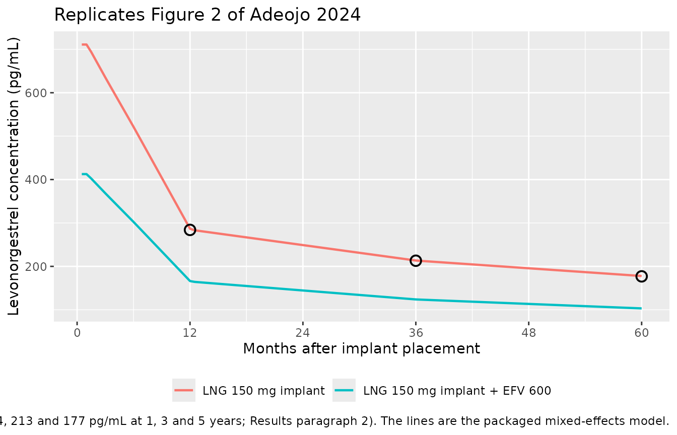
The implant concentrations are an exact arithmetic check
Levonorgestrel’s terminal half-life under this model is roughly a day, so over a release profile that changes on a scale of months the central compartment tracks quasi-steady state, where concentration is simply the release rate divided by clearance. That makes the paper’s three published implant concentrations a direct test of the packaged clearance value.
implant_check <- sim_implant |>
  filter(!is.na(Cc), CONMED_EFV == 0L) |>
  mutate(month = round(time / hours_per_month, 6)) |>
  filter(month %in% c(12, 36, 60)) |>
  transmute(
    month,
    simulated_pg_ml = Cc * 1000,
    # Quasi-steady-state prediction: release rate / CL, with CL = 5.86 L/h.
    rate_ug_day     = approx(release_anchor$month, release_anchor$rate_ug_day,
                             xout = month, rule = 2)$y,
    qss_pg_ml       = rate_ug_day / (5.86 * 24) * 1000
  ) |>
  left_join(published_fig2 |> select(month, published_pg_ml = conc_pg_ml),
            by = "month") |>
  mutate(pct_diff = 100 * (simulated_pg_ml - published_pg_ml) / published_pg_ml)

implant_check |>
  rename(
    "Month"                          = month,
    "Release rate (ug/day)"          = rate_ug_day,
    "Rate / CL (pg/mL)"              = qss_pg_ml,
    "Simulated (pg/mL)"              = simulated_pg_ml,
    "Published (pg/mL)"              = published_pg_ml,
    "% difference"                   = pct_diff
  ) |>
  knitr::kable(
    digits  = 1,
    caption = paste(
      "The packaged model's implant concentrations against the values",
      "Adeojo 2024 reports for its PBPK model. The 'Rate / CL' column shows",
      "that the published numbers are recovered to within rounding by",
      "dividing the Table 1 release rate by the model's clearance of",
      "5.86 L/h - the two models agree here by construction, because the",
      "PBPK model's intrinsic clearance was set by retrograde determination",
      "to match this MEM."
    )
)| Month | Simulated (pg/mL) | Release rate (ug/day) | Rate / CL (pg/mL) | Published (pg/mL) | % difference |
|---|---|---|---|---|---|
| 12 | 286.8 | 40 | 284.4 | 284 | 1.0 |
| 36 | 213.5 | 30 | 213.3 | 213 | 0.2 |
| 60 | 177.8 | 25 | 177.8 | 177 | 0.5 |
Efavirenz effect on the implant route
implant_ratio <- sim_implant |>
  filter(!is.na(Cc), time > 0) |>
  select(treatment, time, Cc) |>
  pivot_wider(names_from = treatment, values_from = Cc) |>
  mutate(ratio = `LNG 150 mg implant + EFV 600` / `LNG 150 mg implant`)

summary(implant_ratio$ratio)
#>    Min. 1st Qu.  Median    Mean 3rd Qu.    Max.
#>  0.5796  0.5802  0.5802  0.5801  0.5802  0.5802
The packaged model predicts implant concentrations with efavirenz that are a constant 58.0% of control, which is exactly the ratio of the two clearance values, 5.86 / 10.1 = 0.580. The paper’s PBPK model predicts 68% of control (Results, paragraph 2). The two disagree, and the disagreement is real rather than a transcription error: the MEM estimates a single time-constant clearance for the efavirenz condition, whereas the Simcyp model applies a time-varying, saturable CYP3A4 induction that has not reached its full effect at every simulated time point. This is discussed further below.
Assumptions and deviations
- The Simcyp PBPK model is deliberately not packaged. Adeojo 2024 Section 2.1 states that the model was built with the Simcyp v19.1 “minimum PKPD” option using “physiologic parameters selected for women ages 18 to 45 years and an average weight of 67.3 kg”, and that “for efavirenz PK and enzyme induction effects, we used model parameters that were included in the software”. Table 1 gives eight levonorgestrel-specific inputs (blood-to-plasma ratio, fraction unbound, CYP3A4 intrinsic clearance, microsomal fraction unbound, human liver microsome elimination, Q, Vss, and the implant release rates). No organ volumes, blood flows, enzyme abundances, gut-model parameters, or efavirenz induction parameters (Indmax, IndC50) are reported anywhere in the article or its supplement, and no ODEs are written out. Reconstructing them would require substituting platform defaults that no available source states, so the PBPK model is documented here rather than approximated. The MEM captures the paper’s levonorgestrel disposition and its efavirenz interaction in full.
- The implant release-rate profile is an event-table input, not a model parameter. Table 1 tabulates the rate at six time points and the Introduction supplies a seventh at 5 years; the values between anchors are linearly interpolated here and delivered as constant-rate infusions of a tenth of a month each, with the rate evaluated at each segment’s midpoint. The authors label three of the six Table 1 entries as interpolated themselves (footnote b), so the underlying profile is itself an interpolation of the Jadelle release data in their reference [8]. A different interpolation scheme would move the between-anchor concentrations slightly but not the anchor values, which is where the validation above is anchored. The segment length is not cosmetic: because the drug’s half-life is about a day, a constant-rate segment reports the release rate at its own midpoint, so coarse (monthly) segments read a stale rate wherever the profile is declining steeply and overshoot the published 1-year concentration by 14%. Tenth-of-a-month segments bring all three published anchors within 1%.
- The route by which the implant enters the model is inferred, not stated. Section 2.2 says only that the MEM used “first-order absorption for oral dosing only”, and Table 1 footnote a states that the tabulated release rates are the amounts reaching systemic circulation. Together these imply that the implant input enters the central compartment directly with no bioavailability term, which is how it is encoded. The exact recovery of the paper’s 284, 213 and 177 pg/mL implant concentrations in the check above confirms this reading: any bioavailability factor on the implant route would scale all three away from the published values.
-
The between-study random effect is encoded as
log-normal. Supplementary Table S2 reports the inter-study
variability of oral bioavailability as 21.2% without stating the
transformation NONMEM used, so it is read as a coefficient of variation
on a log-normal distribution and converted with
omega^2 = log(1 + CV^2). One consequence is worth knowing before using the random effect: with a typical bioavailability of 0.837, a log-normal effect of this size puts roughly a fifth of simulated studies above a bioavailability of 1. Simulations of typical-value behaviour (including every validation in this vignette) userxode2::zeroRe()and are unaffected. -
The fixed absorption rate constant does not quite deliver
the Tmax its footnote cites. Supplementary Table S2 fixes
kaat 4.15 /h and justifies the choice as a “value expected to give tmax of approximately 1-1.5 h, consistent with published observations”. Simulating the packaged model puts the peak at the 0.75 h sampling point, with the underlying continuous maximum near 0.63 h. The discrepancy is in the source, not the transcription. Pairingka= 4.15 /h with the model’s terminal rate constant (beta of about 0.029 /h, a 23.6 h half-life) does give a Tmax of about 1.2 h, which is presumably where the footnote’s figure comes from; but the published model is two-compartment, and its rapid distribution phase (alpha of about 0.39 /h) governs the early profile and pulls the actual peak forward. The value is encoded as published, withfixed()recording that it was not estimated. - The efavirenz covariate is a single binary indicator with no dose information. Both pooled trials that used efavirenz used 600 mg once daily, so the model cannot speak to the 400 mg dose that the paper’s PBPK simulations explore, nor to the CYP2B6-polymorphism exposure range it tests. Those are PBPK-only results.
- The efavirenz effect on the implant route differs from the paper’s PBPK prediction. The packaged model gives 58.0% of control; the paper’s PBPK model gives 68%. Both are reported here without adjustment. The MEM’s single constant clearance for the efavirenz condition was estimated largely from the Carten 2012 oral crossover, whereas the PBPK model applies Simcyp’s time-varying saturable CYP3A4 induction. The paper itself notes (Discussion) that its PBPK predictions in the presence of efavirenz are higher than the Scarsi 2016 observations even though those data were in the MEM reference set, so the two models are known to disagree in this direction. No parameter was tuned to close the gap.
-
The covariate effects are derived, not transcribed.
Supplementary Table S2 reports the efavirenz condition as a second
absolute value for clearance and for bioavailability rather than as a
coefficient. The registry’s linear-deviation form needs a fraction, so
e_conmed_efv_clande_conmed_efv_fdepotare computed from the two published point estimates in each pair. Both reproduce the published efavirenz value exactly: 5.86 x (1 + 0.7235) = 10.1 L/h and 0.837 x (1 - 0.3632) = 0.533. - Vss in Table 1 and the supplement differ slightly. Table 1 reports Vss as 2.27 L/kg from the MEM, which at the stated 67.3 kg average weight is 152.8 L, whereas Supplementary Table S2 gives Vcentral + Vperipheral = 49.5 + 105 = 154.5 L (2.30 L/kg). The supplement’s compartment-level values are used, since they are the parameters the model was fit with; the Table 1 entry is a rounded restatement prepared as a PBPK model input.
- Residual error describes study means, not individual concentrations. The additive 0.214 ng/mL and proportional 8.4% terms quantify how far each trial’s mean profile fell from the model prediction. Simulating with residual error on will not reproduce the scatter of individual patient samples.
- No between-subject variability exists in this model. The source had no individual-level data, so the packaged model cannot generate a conventional VPC or individual concentration predictions.