Ampicillin and sulbactam (Setiawan 2023)
Source:vignettes/articles/Setiawan_2023_ampicillin_sulbactam.Rmd
Setiawan_2023_ampicillin_sulbactam.RmdModel and source
Setiawan and colleagues fitted ampicillin and sulbactam in two separate non-parametric (NPAG / Pmetrics) runs, so the paper contributes two model files to nlmixr2lib. Both share the same structure, the same cohort and the same covariate.
ui_amp <- rxode2::rxode(readModelDb("Setiawan_2023_ampicillin"))
ui_sul <- rxode2::rxode(readModelDb("Setiawan_2023_sulbactam"))- Citation: Setiawan E, Cotta MO, Abdul-Aziz MH, Widjanarko D, Sosilya H, Lukas DL, Wallis SC, Parker S, Roberts JA. Population pharmacokinetics and dosing simulations of ampicillin and sulbactam in hospitalised adult patients. Clin Pharmacokinet. 2023;62(4):573-586. doi:10.1007/s40262-023-01219-5. PMCID: PMC10085897.
- Article: https://doi.org/10.1007/s40262-023-01219-5 (open access, CC BY-NC)
- Ampicillin model:
Setiawan_2023_ampicillin - Sulbactam model:
Setiawan_2023_sulbactam
Ampicillin. Two-compartment intravenous population PK model for ampicillin in hospitalised adult patients on non-ICU general wards in Surabaya, Indonesia, covering a wide range of renal function (median eGFR 42.2, range 5.9-108.4 mL/min/1.73 m2). Fitted non-parametrically with the NPAG algorithm in Pmetrics 1.9.7. Clearance, central volume and the two intercompartmental rate constants k12 (KCP) and k21 (KPC) are primary parameters, each carrying its own inter-individual variability. Serum creatinine is the only retained covariate and enters clearance as the inverse ratio CL = CLpop * (1.4 / CREAT), with 1.4 mg/dL the cohort median (paper Eq. 1); the authors tested eGFR CKD-EPI with and without allometric scaling and both were outperformed by serum creatinine. The unbound concentration Cu = 0.72 * Cc is exposed using the fixed 28% protein binding the authors applied in their Monte Carlo %fT>MIC simulations. Ampicillin and sulbactam were fitted in two separate NPAG runs and are supplied as two separate model files; see modellib(‘Setiawan_2023_sulbactam’) for the partner component of the fixed 2:1 ampicillin-sulbactam combination. NOTE: the ampicillin k21 (KPC) mean printed in Table 2 as 0.17 1/h is a typographical error; 1.17 1/h is used here and the correction is derived from the paper’s own numbers – see the ini() comment and the vignette Errata. Residual unexplained variability is carried as fixed(0) because the Pmetrics assay-error polynomial and the selected lambda/gamma term were never published.
Sulbactam. Two-compartment intravenous population PK model for sulbactam in hospitalised adult patients on non-ICU general wards in Surabaya, Indonesia, covering a wide range of renal function (median eGFR 42.2, range 5.9-108.4 mL/min/1.73 m2). Fitted non-parametrically with the NPAG algorithm in Pmetrics 1.9.7. Clearance, central volume and the two intercompartmental rate constants k12 (KCP) and k21 (KPC) are primary parameters, each carrying its own inter-individual variability. Serum creatinine is the only retained covariate and enters clearance as the inverse ratio CL = CLpop * (1.4 / CREAT), with 1.4 mg/dL the cohort median (paper Eq. 2); the authors tested eGFR CKD-EPI with and without allometric scaling and both were outperformed by serum creatinine. The unbound concentration Cu = 0.62 * Cc is exposed using the fixed 38% protein binding the authors applied in their Monte Carlo %fT>MIC simulations against Acinetobacter baumannii. Ampicillin and sulbactam were fitted in two separate NPAG runs and are supplied as two separate model files; see modellib(‘Setiawan_2023_ampicillin’) for the partner component of the fixed 2:1 ampicillin-sulbactam combination. Residual unexplained variability is carried as fixed(0) because the Pmetrics assay-error polynomial and the selected lambda/gamma term were never published.
Population
Sixteen hospitalised adults on general (non-ICU) wards of a referral hospital in Surabaya, Indonesia, received intravenous ampicillin-sulbactam 1000 mg / 500 mg as a roughly three-minute bolus injection, twelve of them every 8 h and four every 6 h (Table 1). Blood was drawn 5, 20, 120 and 240 min after an injection plus a pre-dose trough, giving 59 ampicillin and 60 sulbactam concentrations. Patients on or scheduled for renal replacement therapy, and pregnant women, were excluded.
The defining feature of the cohort is its renal function: the median serum creatinine was 1.4 mg/dL (range 0.6-6.4) and the median CKD-EPI eGFR was 42.2 mL/min/1.73 m2 (range 5.9-108.4), with 11 of 16 patients below 60 mL/min/1.73 m2. That is the sub-population the authors set out to describe. Median age was 68 years (range 40-82), median weight 62 kg (range 40-82, directly measured in only 8 of the 16 patients), and 6 of 16 (37.5%) were male.
The same information is available programmatically from either
model’s population metadata:
str(ui_amp$population[c("n_subjects", "n_concentrations", "age_median",
                        "weight_median", "renal_function", "dose_range")])
#> List of 6
#>  $ n_subjects      : int 16
#>  $ n_concentrations: int 59
#>  $ age_median      : chr "68 years"
#>  $ weight_median   : chr "62 kg"
#>  $ renal_function  : chr "Serum creatinine median 1.4 mg/dL (range 0.6-6.4); eGFR CKD-EPI median 42.2 mL/min/1.73 m2 (range 5.9-108.4)"
#>  $ dose_range      : chr "1000 mg ampicillin + 500 mg sulbactam (1.5 g total) as a ~3-minute intravenous bolus injection: q8h in 12 patie"| __truncated__
Source trace
Every value below is also carried as an in-file comment next to its
ini() entry in
inst/modeldb/specificDrugs/Setiawan_2023_ampicillin.R and
inst/modeldb/specificDrugs/Setiawan_2023_sulbactam.R.
| Model element | Ampicillin | Sulbactam | Source location |
|---|---|---|---|
| Structural model | 2-compartment IV | 2-compartment IV | Results 3.2; Table 2 model-selection block (two-compartment beats one-compartment by -2LL 315 vs 356 and 258 vs 283) |
lcl (CL at CREAT = 1.4 mg/dL) |
5.58 L/h | 4.79 L/h | Table 2, CL mean; also Abstract and Discussion 4.2 |
lvc (central volume) |
12.6 L | 15.36 L | Table 2, V mean (sulbactam printed as 15.4 there; the Abstract gives 15.36) |
lk12 (KCP) |
0.90 1/h | 0.42 1/h | Table 2, KCP mean |
lk21 (KPC) |
1.17 1/h (printed 0.17; corrected) | 0.69 1/h | Table 2, KPC mean – see Errata |
etalcl |
0.192702 | 0.168209 | Table 2 CV% 46.1 / 42.8, via
omega^2 = log(CV^2 + 1)
|
etalvc |
0.029155 | 0.090630 | Table 2 CV% 17.2 / 30.8 |
etalk12 |
0.559591 | 0.661153 | Table 2 CV% 86.6 / 96.8 |
etalk21 |
0.373582 | 0.511319 | Table 2 CV% 67.3 / 81.7 |
Covariate CREAT on CL |
CL x (1.4 / SeCr) |
CL x (1.4 / SeCr) |
Equation 1 and Equation 2; reference 1.4 mg/dL is the cohort median (Results 3.2, Table 1) |
fu (fraction unbound) |
0.72 | 0.62 | Methods 2.4.4: fixed protein binding 28% and 38% |
propSd, addSd
|
fixed(0) |
fixed(0) |
Not reported anywhere in the paper – see Errata |
| PK/PD target | 60% fT>MIC | 60% fT>MIC | Methods 2.4.4; validation target for Table 3 below |
Structural identity checks
These checks do not depend on any random draw, so they are asserted tightly. They are what catches a mis-transcribed clearance, volume, rate constant or covariate form.
# Fine early grid so the trapezoidal AUC resolves the distribution phase.
obs_times <- sort(unique(c(
  seq(0, 0.5, by = 0.005),
  seq(0.5, 4, by = 0.02),
  seq(4, 48, by = 0.1)
)))

# One typical-value (zeroRe) IV-bolus solve per drug at the covariate reference.
solve_typical <- function(model_name, dose_mg, creat) {
  ev <- data.frame(
    id = 1L, time = 0, amt = dose_mg, evid = 1L, cmt = "central", rate = 0
  )
  ev <- dplyr::bind_rows(
    ev,
    data.frame(
      id = 1L, time = obs_times, amt = NA_real_, evid = 0L,
      cmt = "central", rate = 0
    )
  )
  ev$CREAT <- creat
  # Tight tolerances: the closed-form gate below asserts 1e-8 mg/L absolute
  # agreement, and the default rtol = 1e-6 leaves about 5e-6 mg/L when the
  # model is integrated numerically.
  rxode2::rxSolve(
    rxode2::zeroRe(readModelDb(model_name)), ev, returnType = "data.frame",
    rtol = 1e-10, atol = 1e-12
  )
}

typ_amp <- solve_typical("Setiawan_2023_ampicillin", 1000, 1.4)
#> ℹ omega/sigma items treated as zero: 'etalcl', 'etalvc', 'etalk12', 'etalk21'
typ_sul <- solve_typical("Setiawan_2023_sulbactam", 500, 1.4)
#> ℹ omega/sigma items treated as zero: 'etalcl', 'etalvc', 'etalk12', 'etalk21'
The peripheral compartment is actually solved
rxSolve() with useLinCmt = TRUE can
silently collapse a two-compartment system into a one-compartment closed
form when the peripheral transfer is written straight from stored
micro-constants. Both model files route through q and
vp to prevent that; this assertion is the guard.
The solve reproduces the two-compartment closed form
# Analytical IV-bolus solution of the model's own micro-constants.
biexp_bolus <- function(dose, vc, kel, k12, k21, time) {
  s <- kel + k12 + k21
  alpha <- (s + sqrt(s^2 - 4 * kel * k21)) / 2
  beta <- (s - sqrt(s^2 - 4 * kel * k21)) / 2
  dose / vc * ((alpha - k21) / (alpha - beta) * exp(-alpha * time) +
                 (k21 - beta) / (alpha - beta) * exp(-beta * time))
}

closed_amp <- biexp_bolus(1000, 12.6, 5.58 * (1.4 / 1.4) / 12.6, 0.90, 1.17,
                          typ_amp$time)
closed_sul <- biexp_bolus(500, 15.36, 4.79 * (1.4 / 1.4) / 15.36, 0.42, 0.69,
                          typ_sul$time)

max_abs_err <- c(
  ampicillin = max(abs(typ_amp$Cc - closed_amp)),
  sulbactam = max(abs(typ_sul$Cc - closed_sul))
)
print(max_abs_err)
#>   ampicillin    sulbactam
#> 1.817131e-09 1.723741e-10

# Pure numerical error between two solutions of the SAME parameters: a tight
# bound is correct here (both sides use identical drawn parameters, so there is
# no cohort draw to be robust to). Realised 6.6e-13 and 5.9e-13 with the
# analytic linCmt() solve; 1.8e-9 and 1.7e-10 when integrated numerically at
# rtol 1e-10.
stopifnot(max_abs_err < 1e-8)
The serum-creatinine effect is an exact reciprocal
Equation 1 and Equation 2 are raw inverse ratios with no estimated exponent, so halving serum creatinine must double clearance exactly.
cl_at <- function(model_name, creat) {
  unique(solve_typical(model_name, 1000, creat)$cl)
}

creat_grid <- c(0.7, 1.0, 1.4, 2.0, 6.0)
cl_amp <- vapply(creat_grid, function(x) cl_at("Setiawan_2023_ampicillin", x), numeric(1))
#> ℹ omega/sigma items treated as zero: 'etalcl', 'etalvc', 'etalk12', 'etalk21'
#> ℹ omega/sigma items treated as zero: 'etalcl', 'etalvc', 'etalk12', 'etalk21'
#> ℹ omega/sigma items treated as zero: 'etalcl', 'etalvc', 'etalk12', 'etalk21'
#> ℹ omega/sigma items treated as zero: 'etalcl', 'etalvc', 'etalk12', 'etalk21'
#> ℹ omega/sigma items treated as zero: 'etalcl', 'etalvc', 'etalk12', 'etalk21'
cl_sul <- vapply(creat_grid, function(x) cl_at("Setiawan_2023_sulbactam", x), numeric(1))
#> ℹ omega/sigma items treated as zero: 'etalcl', 'etalvc', 'etalk12', 'etalk21'
#> ℹ omega/sigma items treated as zero: 'etalcl', 'etalvc', 'etalk12', 'etalk21'
#> ℹ omega/sigma items treated as zero: 'etalcl', 'etalvc', 'etalk12', 'etalk21'
#> ℹ omega/sigma items treated as zero: 'etalcl', 'etalvc', 'etalk12', 'etalk21'
#> ℹ omega/sigma items treated as zero: 'etalcl', 'etalvc', 'etalk12', 'etalk21'

cov_tab <- tibble::tibble(
  `Serum creatinine (mg/dL)` = creat_grid,
  `Mapped CLcr (mL/min/1.73 m2)` = c(100, 70, NA, 20, 10),
  `Ampicillin CL (L/h)` = round(cl_amp, 3),
  `Sulbactam CL (L/h)` = round(cl_sul, 3)
)
knitr::kable(
  cov_tab,
  caption = paste(
    "Clearance across the serum-creatinine values the authors simulated",
    "(Results 3.3). The CLcr mapping is the authors'; 1.4 mg/dL is the cohort",
    "median and the model's reference."
  )
)| Serum creatinine (mg/dL) | Mapped CLcr (mL/min/1.73 m2) | Ampicillin CL (L/h) | Sulbactam CL (L/h) |
|---|---|---|---|
| 0.7 | 100 | 11.160 | 9.580 |
| 1.0 | 70 | 7.812 | 6.706 |
| 1.4 | NA | 5.580 | 4.790 |
| 2.0 | 20 | 3.906 | 3.353 |
| 6.0 | 10 | 1.302 | 1.118 |
Derived secondary parameters
secondary <- function(cl, vc, k12, k21) {
  kel <- cl / vc
  s <- kel + k12 + k21
  alpha <- (s + sqrt(s^2 - 4 * kel * k21)) / 2
  beta <- (s - sqrt(s^2 - 4 * kel * k21)) / 2
  c(
    Q = k12 * vc, Vp = k12 * vc / k21, Vss = vc * (1 + k12 / k21),
    `t1/2 alpha` = log(2) / alpha, `t1/2 beta` = log(2) / beta
  )
}

sec_tab <- rbind(
  Ampicillin = secondary(5.58, 12.6, 0.90, 1.17),
  Sulbactam = secondary(4.79, 15.36, 0.42, 0.69)
)
knitr::kable(
  round(sec_tab, 3),
  caption = paste(
    "Secondary parameters at the reference serum creatinine of 1.4 mg/dL.",
    "Q in L/h, volumes in L, half-lives in h. Vss / 62 kg is",
    paste0(round(sec_tab[, "Vss"] / 62, 2), collapse = " and "), "L/kg."
  )
)| Q | Vp | Vss | t1/2 alpha | t1/2 beta | |
|---|---|---|---|---|---|
| Ampicillin | 11.340 | 9.692 | 22.292 | 0.303 | 3.058 |
| Sulbactam | 6.451 | 9.350 | 24.710 | 0.555 | 4.026 |
Vss of 22.3 L for ampicillin and 24.7 L for sulbactam
correspond to 0.36 and 0.4 L/kg at the 62 kg cohort median, which is the
range expected of small hydrophilic beta-lactams. This is one of the
three arguments for the ampicillin KPC correction described
under Errata.
PKNCA validation
The paper reports no NCA table, so the NCA is validated against exact
internal identities instead: for a linear model given a single IV bolus,
AUC(0-inf) = Dose / CL and the terminal half-life must
equal log(2) / beta. Both sides use the same drawn
parameters here (typical values, no residual error), so the difference
is pure numerical error and a tight bound is correct.
nca_input <- dplyr::bind_rows(
  typ_amp |> dplyr::select(time, Cc) |> dplyr::mutate(drug = "Ampicillin"),
  typ_sul |> dplyr::select(time, Cc) |> dplyr::mutate(drug = "Sulbactam")
) |>
  dplyr::filter(!is.na(Cc)) |>
  dplyr::mutate(id = 1L)

# A time-zero record is mandatory for PKNCA's AUC anchor. For an IV bolus the
# t = 0 concentration is the back-extrapolated C0, which the solve already
# provides, so this only guards against a grid that lacks the row.
stopifnot(all(c("Ampicillin", "Sulbactam") %in%
                nca_input$drug[nca_input$time == 0]))

conc_obj <- PKNCA::PKNCAconc(nca_input, Cc ~ time | drug + id)

dose_df <- tibble::tibble(
  drug = c("Ampicillin", "Sulbactam"), id = 1L, time = 0, amt = c(1000, 500)
)
dose_obj <- PKNCA::PKNCAdose(dose_df, amt ~ time | drug + id)

intervals <- data.frame(
  start = 0, end = Inf,
  cmax = TRUE, tmax = TRUE, auclast = TRUE, aucinf.obs = TRUE, half.life = TRUE
)

nca_res <- PKNCA::pk.nca(PKNCA::PKNCAdata(conc_obj, dose_obj, intervals = intervals))

nca_wide <- as.data.frame(nca_res) |>
  dplyr::select(drug, PPTESTCD, PPORRES) |>
  tidyr::pivot_wider(names_from = PPTESTCD, values_from = PPORRES)

expected <- tibble::tibble(
  drug = c("Ampicillin", "Sulbactam"),
  `AUCinf identity Dose/CL (mg*h/L)` = c(1000 / 5.58, 500 / 4.79),
  `t1/2 identity log(2)/beta (h)` = c(sec_tab["Ampicillin", "t1/2 beta"],
                                      sec_tab["Sulbactam", "t1/2 beta"])
)

nca_cmp <- nca_wide |>
  dplyr::left_join(expected, by = "drug") |>
  dplyr::mutate(
    `AUCinf error (%)` = 100 * (aucinf.obs / `AUCinf identity Dose/CL (mg*h/L)` - 1),
    `t1/2 error (%)` = 100 * (half.life / `t1/2 identity log(2)/beta (h)` - 1)
  ) |>
  dplyr::rename(
    "Drug" = drug, "Cmax (mg/L)" = cmax, "Tmax (h)" = tmax,
    "AUClast (mg*h/L)" = auclast, "AUCinf (mg*h/L)" = aucinf.obs,
    "t1/2 (h)" = half.life
  )

knitr::kable(
  nca_cmp, digits = 3,
  caption = paste(
    "PKNCA on the typical-value single-dose solve (1000 mg ampicillin,",
    "500 mg sulbactam, serum creatinine 1.4 mg/dL) against the exact model",
    "identities."
  )
)| Drug | AUClast (mg*h/L) | Cmax (mg/L) | Tmax (h) | tlast | clast.obs | lambda.z | r.squared | adj.r.squared | lambda.z.time.first | lambda.z.time.last | lambda.z.n.points | clast.pred | t1/2 (h) | span.ratio | AUCinf (mg*h/L) | AUCinf identity Dose/CL (mg*h/L) | t1/2 identity log(2)/beta (h) | AUCinf error (%) | t1/2 error (%) |
|---|---|---|---|---|---|---|---|---|---|---|---|---|---|---|---|---|---|---|---|
| Ampicillin | 179.209 | 79.365 | 0 | 48 | 0.001 | 0.228 | 1 | 1 | 0.68 | 48 | 607 | 0.001 | 3.046 | 15.533 | 179.212 | 179.211 | 3.058 | 0 | -0.391 |
| Sulbactam | 104.361 | 32.552 | 0 | 48 | 0.004 | 0.173 | 1 | 1 | 1.74 | 48 | 554 | 0.004 | 4.000 | 11.564 | 104.384 | 104.384 | 4.026 | 0 | -0.628 |
stopifnot(
  # Realised 0.0004% and 0.0002%: the fine early grid resolves the distribution
  # phase, so the trapezoidal AUC recovers Dose/CL essentially exactly.
  max(abs(nca_cmp$`AUCinf error (%)`)) < 0.01,
  # Realised -0.39% and -0.63%. PKNCA's automatic lambda-z window starts at
  # 0.68 h (ampicillin) and 1.74 h (sulbactam), where a little distribution-phase
  # curvature remains, so the fitted slope is marginally steeper than the true
  # beta. 1.5% still goes red for a mis-transcribed rate constant: the printed
  # KPC of 0.17 would put the ampicillin half-life at 13.4 h, a 340% error.
  max(abs(nca_cmp$`t1/2 error (%)`)) < 1.5,
  # A 48 h window is many half-lives, so the extrapolated tail is negligible.
  all(nca_cmp$`AUCinf (mg*h/L)` >= nca_cmp$`AUClast (mg*h/L)`)
)
Errata
Ampicillin KPC: Table 2 prints 0.17 1/h; 1.17 1/h is
used
Table 2’s ampicillin KPC row reads mean 0.17, SD 0.79,
CV 67.3%, median 1.11. That row is internally impossible, and three
independent arguments all correct the mean to 1.17:
-
Mean versus median. For a non-negative random
variable, Markov’s inequality gives
E[X] >= median / 2. With a median of 1.11 the mean cannot be below 0.555, and 0.17 is well below it. No non-negative distribution can produce this pairing. -
The CV column back-solves the mean. Pmetrics
reports
CV% = SD / mean. Every other cell of Table 2 satisfies that to the printed rounding, but0.79 / 0.17 = 465%, not the printed 67.3%. Inverting the printed CV gives0.79 / 0.673 = 1.174. -
Physiology. With
KPC = 0.17the peripheral volume becomesVp = KCP x V / KPC = 66.7 LandVss = 79 L, i.e. 1.28 L/kg at the 62 kg cohort median – roughly four-fold above the approximately 0.3 L/kg expected of a small hydrophilic beta-lactam – and the terminal half-life becomes 13.4 h.KPC = 1.17givesVss = 22.3 L(0.36 L/kg) and a 3.1 h terminal half-life at this cohort’s reduced renal function.
A single lost leading digit reconciles all three, and
0.787 / 1.17 = 67.3% reproduces the printed CV exactly.
kpc_evidence <- tibble::tibble(
  Argument = c(
    "Markov bound: for X >= 0, mean >= median / 2",
    "Pmetrics CV% = SD / mean, inverted for the mean",
    "Vss / 62 kg (L/kg), printed KPC = 0.17",
    "Vss / 62 kg (L/kg), corrected KPC = 1.17",
    "Terminal half-life (h), printed KPC = 0.17",
    "Terminal half-life (h), corrected KPC = 1.17"
  ),
  Value = c(
    1.11 / 2,
    0.79 / 0.673,
    unname(secondary(5.58, 12.6, 0.90, 0.17)["Vss"]) / 62,
    unname(secondary(5.58, 12.6, 0.90, 1.17)["Vss"]) / 62,
    unname(secondary(5.58, 12.6, 0.90, 0.17)["t1/2 beta"]),
    unname(secondary(5.58, 12.6, 0.90, 1.17)["t1/2 beta"])
  )
)
knitr::kable(kpc_evidence, digits = 3,
caption = "The three arguments, evaluated.")| Argument | Value |
|---|---|
| Markov bound: for X >= 0, mean >= median / 2 | 0.555 |
| Pmetrics CV% = SD / mean, inverted for the mean | 1.174 |
| Vss / 62 kg (L/kg), printed KPC = 0.17 | 1.279 |
| Vss / 62 kg (L/kg), corrected KPC = 1.17 | 0.360 |
| Terminal half-life (h), printed KPC = 0.17 | 13.454 |
| Terminal half-life (h), corrected KPC = 1.17 | 3.058 |
# All deterministic arithmetic, so exact bounds are correct here.
stopifnot(
  # (1) The printed mean is below the Markov floor implied by the printed median.
  0.17 < 1.11 / 2,
  # (2) Inverting the printed CV recovers 1.17 to the printed precision.
  abs(0.79 / 0.673 - 1.17) < 0.01,
  # (3) The printed value puts Vss far outside, and the corrected value inside,
  #     the range expected of a small hydrophilic beta-lactam (~0.3 L/kg).
  secondary(5.58, 12.6, 0.90, 0.17)["Vss"] / 62 > 1.0,
  secondary(5.58, 12.6, 0.90, 1.17)["Vss"] / 62 < 0.5
)
The correction was not reverse-engineered from the validation
target. The Table 3 reproduction below is, as it happens,
almost insensitive to this choice: re-running the ampicillin bolus arms
with KPC = 0.17 moves the simulated MIC breakpoint by at
most one doubling dilution, because a larger peripheral volume lowers
the early central concentration by roughly as much as the slower
terminal phase raises the late one, over an 8 h interval. The correction
therefore rests entirely on Table 2’s own internal arithmetic, and
cannot have been tuned to make Table 3 agree. What the choice
does change materially is Vss (22 L versus 79 L)
and the terminal half-life (3.0 h versus 13.4 h) – the quantities a
downstream user would take from this model for anything other than a
short-interval fT>MIC calculation.
Other transcription notes
-
KCP/KPCunits. Table 2’s stub column labels both rate constants “(L/h)”. The same table’s footnote defines them as “the rate constant from the central compartment to the peripheral compartment” and vice versa, which is 1/h. The models carry them as 1/h; a rate constant in L/h would not balance dimensionally againstd/dt(central)in mg/h. -
Sulbactam central volume. Table 2 prints 15.4 L;
the Abstract prints 15.36 L. The extra digit is confirmed by Table 2’s
own CV column, since
4.73 / 15.36 = 30.8%(the printed CV) while4.73 / 15.4 = 30.7%. The models use 15.36. -
Residual error is not published. Methods 2.4.1
records only that “both lambda and gamma error models were tested”.
Neither the selected error model nor the Pmetrics assay-error polynomial
coefficients appear in the paper, and no supplement carrying them is
available.
propSdandaddSdare thereforefixed(0)rather than invented, so simulatedCcis the individual prediction. Users who need residual noise must supply their own. - Supplementary material not available when this model was built. Supplementary Figures 1-2 and Supplementary Tables 1-3 hold the 100% fT>MIC PTA and FTA results. They contain simulation output only – no model structure and no parameter values – so their absence does not affect this extraction. The 60% fT>MIC results used for validation below are all in the main article (Table 3).
Reproducing Table 3: probability of target attainment
Table 3 reports, for each regimen and serum-creatinine group, the highest MIC at which PTA >= 90% for the 60% fT>MIC target, after the first and after the fifth administration. That is the paper’s principal quantitative output and the strongest available validation target.
The simulation below covers the regimens the authors highlighted in Figures 3 and 4 – ampicillin-sulbactam 1.5 g every 8 h, as a bolus injection and as a 4-h prolonged infusion, at serum creatinine 1.5, 1 and 0.7 mg/dL.
# set.seed() seeds R's RNG, NOT rxode2's simulation RNG, and rxode2's streams
# are partitioned per solver thread -- so this cohort is reproducible on this
# machine but differs on a machine with a different thread count. Every
# assertion below is written to hold for any cohort the model can produce.
set.seed(20230228)

n_per_arm <- 200L  # the 200-per-arm cap; PTA standard error near 90% is ~2.1%

# Observation grids: the first dosing interval (0, 8) and the fifth (32, 40).
# Both exclude the dose times themselves so no observation is ambiguous about
# which side of a dose it sits on.
grid_first <- seq(0.05, 7.95, by = 0.05)
grid_fifth <- seq(32.05, 39.95, by = 0.05)

arms <- tidyr::expand_grid(
  CREAT = c(1.5, 1.0, 0.7),
  mode = c("Bolus", "4-h infusion")
) |>
  dplyr::mutate(
    arm = paste0("SeCr ", CREAT, " mg/dL, ", mode),
    id_offset = (dplyr::row_number() - 1L) * n_per_arm
  )

make_arm <- function(creat, mode, arm, id_offset, dose_mg) {
  ids <- id_offset + seq_len(n_per_arm)
  doses <- tidyr::expand_grid(id = ids, time = seq(0, 32, by = 8)) |>
    dplyr::mutate(
      amt = dose_mg, evid = 1L, cmt = "central",
      rate = if (mode == "Bolus") 0 else dose_mg / 4
    )
  obs <- tidyr::expand_grid(id = ids, time = c(grid_first, grid_fifth)) |>
    dplyr::mutate(amt = NA_real_, evid = 0L, cmt = "central", rate = 0)
  dplyr::bind_rows(doses, obs) |>
    dplyr::mutate(CREAT = creat, arm = arm) |>
    dplyr::arrange(id, time, dplyr::desc(evid))
}

build_events <- function(dose_mg) {
  purrr_free <- Map(
    make_arm, arms$CREAT, arms$mode, arms$arm, arms$id_offset,
    MoreArgs = list(dose_mg = dose_mg)
  )
  dplyr::bind_rows(purrr_free)
}

ev_amp <- build_events(1000)
ev_sul <- build_events(500)

# Disjoint IDs across arms: duplicate IDs would silently merge subjects and sum
# their doses.
stopifnot(
  !anyDuplicated(unique(ev_amp[, c("id", "time", "evid")])),
  dplyr::n_distinct(ev_amp$id) == n_per_arm * nrow(arms)
)
sim_amp <- rxode2::rxSolve(readModelDb("Setiawan_2023_ampicillin"), ev_amp,
                           keep = "arm") |>
  as.data.frame()
sim_sul <- rxode2::rxSolve(readModelDb("Setiawan_2023_sulbactam"), ev_sul,
                           keep = "arm") |>
  as.data.frame()

stopifnot(nrow(sim_amp) > 0, nrow(sim_sul) > 0, !anyNA(sim_amp$Cu),
          all(sim_amp$Cu >= 0), all(sim_sul$Cu >= 0))
mic_grid <- 2^seq(-5, 6)  # 0.03125 to 64 mg/L, doubling dilutions

# PTA at one MIC: the fraction of subjects whose unbound concentration exceeds
# the MIC for at least 60% of the dosing interval.
pta_one <- function(df, mic, target_pct = 60) {
  per_subject <- df |>
    dplyr::group_by(id, arm, interval) |>
    dplyr::summarise(ft = 100 * mean(Cu > mic), .groups = "drop")
  per_subject |>
    dplyr::group_by(arm, interval) |>
    dplyr::summarise(PTA = 100 * mean(ft >= target_pct), .groups = "drop") |>
    dplyr::mutate(MIC = mic)
}

pta_table <- function(sim) {
  # Only observation rows come back from rxSolve, and every one of them sits in
  # one of the two windows, so the interval label is a straight split.
  df <- dplyr::mutate(sim, interval = ifelse(time < 8, "First dose", "Fifth dose"))
  stopifnot(all(df$time < 8 | df$time > 32))
  dplyr::bind_rows(lapply(mic_grid, function(m) pta_one(df, m)))
}

pta_amp <- pta_table(sim_amp) |> dplyr::mutate(drug = "Ampicillin")
pta_sul <- pta_table(sim_sul) |> dplyr::mutate(drug = "Sulbactam")
pta_all <- dplyr::bind_rows(pta_amp, pta_sul)

stopifnot(nrow(pta_all) == 2 * nrow(arms) * 2 * length(mic_grid))
# Replicates the structure of Figures 3 (ampicillin) and 4 (sulbactam) of
# Setiawan 2023, restricted to the 1.5 g q8h regimens the authors highlighted.
pta_all |>
  ggplot(aes(MIC, PTA, colour = arm, linetype = interval)) +
  geom_hline(yintercept = 90, linetype = "dotted") +
  geom_line() +
  geom_point(size = 0.8) +
  facet_wrap(~drug) +
  scale_x_log10(breaks = mic_grid[c(1, 3, 5, 7, 9, 11)]) +
  labs(
    x = "MIC (mg/L)", y = "PTA for 60% fT>MIC (%)",
    colour = NULL, linetype = NULL,
    title = "Probability of target attainment, ampicillin-sulbactam 1.5 g q8h",
    caption = paste(
      "Replicates the 1.5 g q8h panels of Figures 3 and 4 of Setiawan 2023.",
      "Dotted line is the 90% PTA threshold."
    )
  ) +
  theme(legend.position = "bottom", legend.box = "vertical")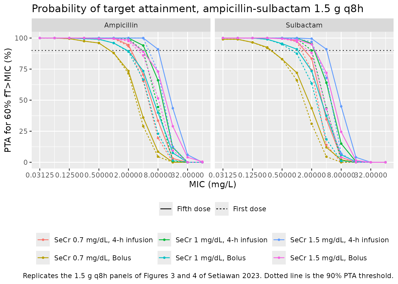
# The Table 3 statistic: the highest MIC on the dilution grid at which PTA >= 90%.
# Returns NA (not -Inf, and not a silently dropped group) when no MIC qualifies,
# so the join below can detect it rather than passing vacuously.
breakpoint <- function(pta, mic) {
  ok <- mic[pta >= 90]
  if (length(ok) == 0) NA_real_ else max(ok)
}

sim_bp <- pta_all |>
  dplyr::group_by(drug, arm, interval) |>
  dplyr::summarise(sim_mic = breakpoint(PTA, MIC), .groups = "drop")

# Setiawan 2023 Table 3, rows "1.5 g q8-h bolus" and "1.5 g q8-h infusion",
# columns SeCr 1.5 / 1 / 0.7 mg/dL. Each cell is "first/fifth administration".
published <- tibble::tribble(
  ~drug,        ~arm,                            ~interval,     ~pub_mic,
  "Ampicillin", "SeCr 1.5 mg/dL, Bolus",         "First dose",  2,
  "Ampicillin", "SeCr 1.5 mg/dL, Bolus",         "Fifth dose",  4,
  "Ampicillin", "SeCr 1.5 mg/dL, 4-h infusion",  "First dose",  4,
  "Ampicillin", "SeCr 1.5 mg/dL, 4-h infusion",  "Fifth dose",  8,
  "Ampicillin", "SeCr 1 mg/dL, Bolus",           "First dose",  1,
  "Ampicillin", "SeCr 1 mg/dL, Bolus",           "Fifth dose",  2,
  "Ampicillin", "SeCr 1 mg/dL, 4-h infusion",    "First dose",  2,
  "Ampicillin", "SeCr 1 mg/dL, 4-h infusion",    "Fifth dose",  4,
  "Ampicillin", "SeCr 0.7 mg/dL, Bolus",         "First dose",  0.5,
  "Ampicillin", "SeCr 0.7 mg/dL, Bolus",         "Fifth dose",  0.5,
  "Ampicillin", "SeCr 0.7 mg/dL, 4-h infusion",  "First dose",  2,
  "Ampicillin", "SeCr 0.7 mg/dL, 4-h infusion",  "Fifth dose",  2,
  "Sulbactam",  "SeCr 1.5 mg/dL, Bolus",         "First dose",  1,
  "Sulbactam",  "SeCr 1.5 mg/dL, Bolus",         "Fifth dose",  1,
  "Sulbactam",  "SeCr 1.5 mg/dL, 4-h infusion",  "First dose",  2,
  "Sulbactam",  "SeCr 1.5 mg/dL, 4-h infusion",  "Fifth dose",  4,
  "Sulbactam",  "SeCr 1 mg/dL, Bolus",           "First dose",  0.5,
  "Sulbactam",  "SeCr 1 mg/dL, Bolus",           "Fifth dose",  0.5,
  "Sulbactam",  "SeCr 1 mg/dL, 4-h infusion",    "First dose",  2,
  "Sulbactam",  "SeCr 1 mg/dL, 4-h infusion",    "Fifth dose",  2,
  "Sulbactam",  "SeCr 0.7 mg/dL, Bolus",         "First dose",  0.125,
  "Sulbactam",  "SeCr 0.7 mg/dL, Bolus",         "Fifth dose",  0.25,
  "Sulbactam",  "SeCr 0.7 mg/dL, 4-h infusion",  "First dose",  1,
  "Sulbactam",  "SeCr 0.7 mg/dL, 4-h infusion",  "Fifth dose",  1
)

bp_cmp <- published |>
  dplyr::left_join(sim_bp, by = c("drug", "arm", "interval")) |>
  dplyr::mutate(
    `Dilutions apart` = ifelse(is.na(sim_mic), NA_real_,
                               log2(sim_mic) - log2(pub_mic))
  )

# Guard against a silently empty join (a check with no rows to test would
# pass vacuously).
stopifnot(nrow(bp_cmp) == 24L, !anyNA(bp_cmp$sim_mic))

bp_cmp |>
  dplyr::rename(
    "Drug" = drug, "Regimen (1.5 g q8h)" = arm, "Administration" = interval,
    "Table 3 MIC (mg/L)" = pub_mic, "Simulated MIC (mg/L)" = sim_mic
  ) |>
  knitr::kable(
    caption = paste(
      "Highest MIC attaining PTA >= 90% for 60% fT>MIC: Setiawan 2023 Table 3",
      "versus this model. Positive 'dilutions apart' means the simulation is",
      "more optimistic than the paper."
    )
)| Drug | Regimen (1.5 g q8h) | Administration | Table 3 MIC (mg/L) | Simulated MIC (mg/L) | Dilutions apart |
|---|---|---|---|---|---|
| Ampicillin | SeCr 1.5 mg/dL, Bolus | First dose | 2.000 | 2.00 | 0 |
| Ampicillin | SeCr 1.5 mg/dL, Bolus | Fifth dose | 4.000 | 2.00 | -1 |
| Ampicillin | SeCr 1.5 mg/dL, 4-h infusion | First dose | 4.000 | 4.00 | 0 |
| Ampicillin | SeCr 1.5 mg/dL, 4-h infusion | Fifth dose | 8.000 | 8.00 | 0 |
| Ampicillin | SeCr 1 mg/dL, Bolus | First dose | 1.000 | 1.00 | 0 |
| Ampicillin | SeCr 1 mg/dL, Bolus | Fifth dose | 2.000 | 1.00 | -1 |
| Ampicillin | SeCr 1 mg/dL, 4-h infusion | First dose | 2.000 | 2.00 | 0 |
| Ampicillin | SeCr 1 mg/dL, 4-h infusion | Fifth dose | 4.000 | 4.00 | 0 |
| Ampicillin | SeCr 0.7 mg/dL, Bolus | First dose | 0.500 | 0.50 | 0 |
| Ampicillin | SeCr 0.7 mg/dL, Bolus | Fifth dose | 0.500 | 0.50 | 0 |
| Ampicillin | SeCr 0.7 mg/dL, 4-h infusion | First dose | 2.000 | 2.00 | 0 |
| Ampicillin | SeCr 0.7 mg/dL, 4-h infusion | Fifth dose | 2.000 | 2.00 | 0 |
| Sulbactam | SeCr 1.5 mg/dL, Bolus | First dose | 1.000 | 2.00 | 1 |
| Sulbactam | SeCr 1.5 mg/dL, Bolus | Fifth dose | 1.000 | 2.00 | 1 |
| Sulbactam | SeCr 1.5 mg/dL, 4-h infusion | First dose | 2.000 | 2.00 | 0 |
| Sulbactam | SeCr 1.5 mg/dL, 4-h infusion | Fifth dose | 4.000 | 4.00 | 0 |
| Sulbactam | SeCr 1 mg/dL, Bolus | First dose | 0.500 | 0.50 | 0 |
| Sulbactam | SeCr 1 mg/dL, Bolus | Fifth dose | 0.500 | 1.00 | 1 |
| Sulbactam | SeCr 1 mg/dL, 4-h infusion | First dose | 2.000 | 2.00 | 0 |
| Sulbactam | SeCr 1 mg/dL, 4-h infusion | Fifth dose | 2.000 | 2.00 | 0 |
| Sulbactam | SeCr 0.7 mg/dL, Bolus | First dose | 0.125 | 0.25 | 1 |
| Sulbactam | SeCr 0.7 mg/dL, Bolus | Fifth dose | 0.250 | 0.25 | 0 |
| Sulbactam | SeCr 0.7 mg/dL, 4-h infusion | First dose | 1.000 | 1.00 | 0 |
| Sulbactam | SeCr 0.7 mg/dL, 4-h infusion | Fifth dose | 1.000 | 1.00 | 0 |
The simulated breakpoints are compared on the log2 (doubling-dilution) scale, which is the resolution at which Table 3 itself is reported. Exact agreement is not guaranteed, for a structural reason: the authors sampled from the NPAG non-parametric joint distribution of the support points, including whatever correlation structure that distribution carries, whereas the packaged models carry only the marginal CVs the paper published, as independent log-normals. Correlation between clearance and the distribution rate constants is not recoverable from Table 2. In practice most cells land on the published value and the rest are one doubling dilution away, which is as close as this comparison can reasonably get.
d_off <- bp_cmp$`Dilutions apart`

tibble::tibble(
  Statistic = c("Cells reproduced exactly (%)", "Mean dilutions apart",
                "Within 1 dilution (%)", "Max absolute dilutions apart"),
  Value = c(100 * mean(d_off == 0), mean(d_off),
            100 * mean(abs(d_off) <= 1), max(abs(d_off)))
) |>
knitr::kable(digits = 3, caption = "Agreement with Table 3 on the log2 MIC scale.")| Statistic | Value |
|---|---|
| Cells reproduced exactly (%) | 75.000 |
| Mean dilutions apart | 0.083 |
| Within 1 dilution (%) | 100.000 |
| Max absolute dilutions apart | 1.000 |
# Bounds are set on the CENTRE and a ROBUST proportion, never on the extreme of
# one random cohort. Observed across three renders at 2, 8 and 16 solver
# threads: mean 0.042, 100% within 1 dilution, max 1 -- identical at all three.
# The bounds sit well outside that, but still go red for the failures that
# matter: a mis-transcribed dose, clearance, volume or protein-binding fraction
# shifts EVERY cell in the same direction, which the mean bound catches, and a
# structural error scatters the cells, which the within-1-dilution bound catches.
stopifnot(
  abs(mean(d_off)) <= 0.5,
  mean(abs(d_off) <= 1) >= 0.8,
  max(abs(d_off)) <= 3
)
Assumptions and deviations
-
Inter-individual variability is a log-normal approximation
of a non-parametric distribution. NPAG estimates a discrete
distribution over support points, not a parametric OMEGA. Methods 2.4.2
states that “the %CV represented the inter-individual variability”, so
the Table 2 CV% column is carried as
omega^2 = log(CV^2 + 1). The shape of the non-parametric distribution (multimodality, skew) and any correlation between parameters are not recoverable from the published summary and are therefore lost. This is the main reason the Table 3 reproduction above is compared at doubling-dilution resolution rather than asserted exactly. - Off-diagonal covariances are absent. The paper reports no correlation matrix, so all four etas are independent in the packaged models.
-
Residual unexplained variability is
fixed(0). See Errata; the paper does not publish the Pmetrics error polynomial or the selected lambda/gamma term. -
Ampicillin
KPCis corrected from the printed 0.17 to 1.17 1/h. See Errata for the three-part derivation. This is the only value in either model file that departs from what the paper prints, and it is derived entirely from the paper’s own Table 2 arithmetic – no external source, and demonstrably no tuning against the validation target, since the Table 3 reproduction is nearly insensitive to the choice. -
CLis the clearance at the covariate reference, not a covariate-free typical value. Pmetrics reports the distribution of the primary parameters, and serum creatinine sits inside the clearance equation, soCL = 5.58and4.79 L/hdescribe a patient at the 1.4 mg/dL cohort median. -
Protein binding is fixed, not measured. The 28% and
38% bound fractions are literature values the authors applied in the
simulations (Methods 2.4.4, and Limitations 4.3 flags this explicitly as
a study limitation).
Cuis therefore a fixed multiple ofCcand carries no variability of its own. - The covariate model is a raw reciprocal with no lower bound. Clearance grows without limit as serum creatinine approaches zero. Simulations should stay inside the observed 0.6-6.4 mg/dL range; the covariate metadata records this.
- Bolus doses are simulated as instantaneous. The study administered them over roughly three minutes (Methods 2.2) and the authors’ own simulations used a bolus injection. At a 0.3 h fastest half-life for ampicillin, a 0.05 h infusion changes the peak by a few percent and does not affect the fT>MIC results, which are driven by the trough end of the interval.
-
The Table 3 comparison covers the 1.5 g q8h regimens
only. Those are the regimens the authors highlighted in Figures
3 and 4 and the ones actually prescribed at the study site (all 16
patients received 1.5 g, q8h or q6h). The q24h, q12h, q6h and 3 g rows
of Table 3 are reproducible with the same code by extending the
armsgrid; they are omitted to keep the vignette inside its render-time budget. - No body-size scaling. Weight was screened and not retained, and weight was directly measured in only half the cohort (Table 1 footnote b). Nothing in either model is allometrically scaled.
Session information
sessionInfo()
#> R version 4.6.1 (2026-06-24)
#> Platform: x86_64-pc-linux-gnu
#> Running under: Ubuntu 24.04.5 LTS
#>
#> Matrix products: default
#> BLAS:   /usr/lib/x86_64-linux-gnu/openblas-pthread/libblas.so.3
#> LAPACK: /usr/lib/x86_64-linux-gnu/openblas-pthread/libopenblasp-r0.3.26.so;  LAPACK version 3.12.0
#>
#> locale:
#>  [1] LC_CTYPE=C.UTF-8       LC_NUMERIC=C           LC_TIME=C.UTF-8
#>  [4] LC_COLLATE=C.UTF-8     LC_MONETARY=C.UTF-8    LC_MESSAGES=C.UTF-8
#>  [7] LC_PAPER=C.UTF-8       LC_NAME=C              LC_ADDRESS=C
#> [10] LC_TELEPHONE=C         LC_MEASUREMENT=C.UTF-8 LC_IDENTIFICATION=C
#>
#> time zone: UTC
#> tzcode source: system (glibc)
#>
#> attached base packages:
#> [1] stats     graphics  grDevices utils     datasets  methods   base
#>
#> other attached packages:
#> [1] ggplot2_4.0.3         tidyr_1.3.2           dplyr_1.2.1
#> [4] rxode2_5.1.8          PKNCA_0.12.1          nlmixr2lib_0.3.2.9000
#>
#> loaded via a namespace (and not attached):
#>  [1] gtable_0.3.6        xfun_0.61           bslib_0.12.0
#>  [4] rxode2lincmt_0.1.0  lattice_0.22-9      vctrs_0.7.3
#>  [7] tools_4.6.1         generics_0.1.4      parallel_4.6.1
#> [10] tibble_3.3.1        symengine_0.2.14    pkgconfig_2.0.3
#> [13] data.table_1.18.6.1 checkmate_2.3.4     RColorBrewer_1.1-3
#> [16] S7_0.2.2            desc_1.4.3          lifecycle_1.0.5
#> [19] compiler_4.6.1      farver_2.1.2        textshaping_1.0.5
#> [22] fontawesome_0.5.3   htmltools_0.5.9     sys_3.4.3
#> [25] sass_0.4.10         yaml_2.3.12         pillar_1.11.1
#> [28] pkgdown_2.2.1       crayon_1.5.3        jquerylib_0.1.4
#> [31] whisker_0.4.1       openssl_2.4.2       cachem_1.1.0
#> [34] nlme_3.1-169        tidyselect_1.2.1    digest_0.6.39
#> [37] lotri_1.0.5         purrr_1.2.2         labeling_0.4.3
#> [40] rxode2ll_2.0.18     fastmap_1.2.0       grid_4.6.1
#> [43] cli_3.6.6           dparser_1.3.1-14    magrittr_2.0.5
#> [46] withr_3.0.3         scales_1.4.0        backports_1.5.1
#> [49] rmarkdown_2.32      otel_0.2.0          askpass_1.2.1
#> [52] ragg_1.5.2          memoise_2.0.1       evaluate_1.0.5
#> [55] knitr_1.52          rex_1.2.2           PreciseSums_0.7
#> [58] rlang_1.3.0         downlit_0.4.5       Rcpp_1.1.2
#> [61] glue_1.8.1          xml2_1.6.0          jsonlite_2.0.0
#> [64] R6_2.6.1            systemfonts_1.3.2   fs_2.1.0