Amlodipine (Courlet 2021) • nlmixr2lib

Model and source

Citation: Courlet P, Guidi M, Alves Saldanha S, Cavassini M, Stoeckle M, Buclin T, Marzolini C, Decosterd LA, Csajka C; Swiss HIV Cohort Study. Population pharmacokinetic modelling to quantify the magnitude of drug-drug interactions between amlodipine and antiretroviral drugs. Eur J Clin Pharmacol. 2021;77:979-987. doi:10.1007/s00228-020-03060-2
Description: One-compartment population PK model for oral amlodipine in adults living with HIV (Courlet 2021), with first-order absorption after a lag time, between-subject variability on apparent clearance only, an additive residual error, and two antiretroviral drug-drug-interaction effects on CL/F: a -49% linear effect of strong CYP3A4-inhibiting ARVs (boosted darunavir, boosted atazanavir, cobicistat-boosted elvitegravir) and a +140% linear effect of efavirenz.
Article: Eur J Clin Pharmacol 2021;77:979-987 (open access)

Courlet et al. pooled sparse therapeutic-monitoring samples from the Swiss HIV Cohort Study (project 815) with a rich-sampling PK study (NCT03515772) to quantify how antiretroviral drugs (ARVs) change the exposure of amlodipine, a CYP3A4 substrate. The final model is a one-compartment model with first-order absorption after a lag time, between-subject variability on apparent clearance only and an additive residual error. Two ARV effects were retained on CL/F:

$CL/F = 17.0 \times (1 - 0.49 \times \mathrm{CYP3A4\ inhibitors}) \times (1 + 1.40 \times \mathrm{efavirenz})$

(Table 2 footnote). In the packaged model the two indicators are the canonical covariates CONMED_CYP3A4_INH_STRONG (ritonavir- or cobicistat-boosted darunavir, ritonavir-boosted atazanavir, cobicistat-boosted elvitegravir) and CONMED_EFV.

Population

The model was developed from 163 amlodipine plasma concentrations in 55 people living with HIV in Lausanne and Basel, Switzerland (Table 1): median age 61 years (IQR 53-70), median body weight 79 kg (IQR 71-91), 75% male. Eight subjects in the rich-sampling study contributed 84 concentrations (8-11 each, up to 28 h post-dose); the cohort subjects contributed 1-3 samples each. Amlodipine was taken at 2.5-10 mg once daily (three subjects 5 mg twice daily) and all subjects were assumed to be at steady state. Of the 163 samples, 36 were drawn under a strong CYP3A4-inhibiting ARV (27 under ritonavir-boosted darunavir) and 7 under efavirenz. Age, sex, body weight, albumin, AST, ALT and creatinine clearance were tested and not retained.

The same information is available programmatically via readModelDb("Courlet_2021_amlodipine")()$population.

Source trace

Equation / parameter	Value	Source location
`lka` (ka)	log(0.69) 1/h	Table 2, ‘ka’
`ltlag` (ALAG)	log(0.87) h	Table 2, ‘ALAG’
`lvc` (V/F)	log(1000) L	Table 2, ‘V/F’
`lcl` (CL/F)	log(17.0) L/h	Table 2, ‘CL/F’
`e_conmed_cyp3a4_inh_strong_cl`	-0.49	Table 2, ‘theta CYP3A4 inhibitors’
`e_conmed_efv_cl`	1.40	Table 2, ‘theta efavirenz’
`etalcl`	0.16246 = log(1 + 0.42^2)	Table 2, ‘BSV CL (CV%)’ = 42
`addSd`	2.85 ng/mL	Table 2, ‘sigma add’
CL/F covariate equation	n/a	Table 2 footnote ‘Final model’
One compartment, first-order absorption with lag	n/a	Results, ‘Structural, statistical and covariate models’
`Cc = 1000 * central / vc`	n/a	mg / L to ng/mL (units of Table 2 and Table 3)

Typical-value checks

The typical-value half-life of amlodipine without interacting ARVs, stated in the Discussion as 40.8 h, follows directly from V/F and CL/F.

mod <- readModelDb("Courlet_2021_amlodipine")
ini_df <- rxode2::rxode(mod)$iniDf
#> ℹ parameter labels from comments will be replaced by 'label()'
theta <- setNames(ini_df$est, ini_df$name)
ka <- exp(theta[["lka"]])
tlag <- exp(theta[["ltlag"]])
vc <- exp(theta[["lvc"]])
cl0 <- exp(theta[["lcl"]])
thalf <- log(2) * vc / cl0
thalf
#> [1] 40.77336
stopifnot(abs(thalf - 40.8) < 0.05)

Steady-state closed form versus the ODE solve

A one-compartment model with first-order absorption and a lag at steady state has a closed form; the ODE solve of the packaged model must reproduce it.

# Steady-state concentration (ng/mL) at time t after a dose, dosing every tau,
# for the typical subject with clearance `cl`. The lag shifts the phase, so
# the time since the last *absorbed* dose is (t - tlag) modulo tau.
css_closed <- function(t, dose, tau, cl) {
  k <- cl / vc
  tp <- (t - tlag) %% tau
  1000 * dose / vc * ka / (ka - k) *
    (exp(-k * tp) / (1 - exp(-k * tau)) - exp(-ka * tp) / (1 - exp(-ka * tau)))
}

ss_events <- function(dose, tau, inh, efv, id = 1L, grid = seq(0, 24, by = 0.25)) {
  n_dose <- 24 / tau
  dplyr::bind_rows(
    data.frame(
      id = id, time = 0, evid = 1L, amt = dose, ii = tau, ss = 1L,
      addl = n_dose - 1L, cmt = "depot"
    ),
    data.frame(
      id = id, time = grid, evid = 0L, amt = 0, ii = 0, ss = 0L,
      addl = 0L, cmt = "central"
    )
  ) |>
    dplyr::mutate(CONMED_CYP3A4_INH_STRONG = inh, CONMED_EFV = efv) |>
    dplyr::arrange(id, time, dplyr::desc(evid))
}

mod_typ <- rxode2::zeroRe(mod)
#> ℹ parameter labels from comments will be replaced by 'label()'
typ_sim <- function(dose, tau, inh, efv) {
  rxode2::rxSolve(
    mod_typ, ss_events(dose, tau, inh, efv),
    rtol = 1e-10, atol = 1e-12, ssRtol = 1e-10, ssAtol = 1e-12, maxsteps = 1e6
  ) |>
    as.data.frame()
}

chk <- typ_sim(5, 24, 0, 0)
#> ℹ omega/sigma items treated as zero: 'etalcl'
cf <- css_closed(chk$time, 5, 24, cl0)
max_rel <- max(abs(chk$Cc / cf - 1))
max_rel
#> [1] 9.260503e-11
stopifnot(max_rel < 1e-6)

Replicating Table 3 and the simulation claims

Table 3 reports the median Cmax, Ctrough (24 h post-dose) and AUC0-24 (computed as dose/CL) of 1000 simulated subjects for the standard 5 mg once-daily regimen and the two proposed alternatives. The Results text adds the exposure changes at 5 mg once daily with each interactor and two further efavirenz regimens (15 mg once daily and 5 mg twice daily, shown in the paper’s supplementary material). The typical-subject values of the packaged model are compared with those medians below.

regimens <- tibble::tribble(
  ~regimen,                         ~dose, ~tau, ~inh, ~efv,
  "5 mg qd alone",                  5,     24,   0,    0,
  "2.5 mg qd + CYP3A4 inhibitor",   2.5,   24,   1,    0,
  "10 mg qd + efavirenz",           10,    24,   0,    1,
  "5 mg qd + CYP3A4 inhibitor",     5,     24,   1,    0,
  "5 mg qd + efavirenz",            5,     24,   0,    1,
  "15 mg qd + efavirenz",           15,    24,   0,    1,
  "5 mg bid + efavirenz",           5,     12,   0,    1
)

typ <- regimens |>
  dplyr::rowwise() |>
  dplyr::mutate(
    sim = list(typ_sim(dose, tau, inh, efv)),
    cmax = max(sim$Cc),
    ctrough = sim$Cc[sim$time == 24],
    auc024 = 1000 * (24 / tau) * dose /
      (cl0 * (1 + theta[["e_conmed_cyp3a4_inh_strong_cl"]] * inh) *
        (1 + theta[["e_conmed_efv_cl"]] * efv))
  ) |>
  dplyr::ungroup() |>
  dplyr::select(-sim)
#> ℹ omega/sigma items treated as zero: 'etalcl'
#> ℹ omega/sigma items treated as zero: 'etalcl'
#> ℹ omega/sigma items treated as zero: 'etalcl'
#> ℹ omega/sigma items treated as zero: 'etalcl'
#> ℹ omega/sigma items treated as zero: 'etalcl'
#> ℹ omega/sigma items treated as zero: 'etalcl'
#> ℹ omega/sigma items treated as zero: 'etalcl'
stopifnot(nrow(typ) == nrow(regimens))

ref <- typ |> dplyr::filter(regimen == "5 mg qd alone")
typ <- typ |>
  dplyr::mutate(
    ratio_cmax = cmax / ref$cmax,
    ratio_ctrough = ctrough / ref$ctrough,
    ratio_auc = auc024 / ref$auc024
  )

published_t3 <- tibble::tribble(
  ~regimen,                         ~cmax, ~ctrough, ~auc024,
  "5 mg qd alone",                  13.6,  10.2,     290.8,
  "2.5 mg qd + CYP3A4 inhibitor",   12.7,  10.9,     285.7,
  "10 mg qd + efavirenz",           13.7,  6.5,      242.3
)

t3 <- published_t3 |>
  dplyr::inner_join(typ, by = "regimen", suffix = c("_paper", "_model"))
stopifnot(nrow(t3) == 3L)
t3 <- t3 |>
  dplyr::mutate(
    pct_cmax = 100 * (cmax_model / cmax_paper - 1),
    pct_ctrough = 100 * (ctrough_model / ctrough_paper - 1),
    pct_auc = 100 * (auc024_model / auc024_paper - 1)
  )

t3 |>
  dplyr::transmute(
    Regimen = regimen,
    "Cmax paper" = cmax_paper, "Cmax model" = round(cmax_model, 1),
    "Ctrough paper" = ctrough_paper, "Ctrough model" = round(ctrough_model, 1),
    "AUC0-24 paper" = auc024_paper, "AUC0-24 model" = round(auc024_model, 1)
  ) |>
  knitr::kable(caption = "Table 3 medians (ng/mL, ng*h/mL) against the typical subject of the packaged model.")

Table 3 medians (ng/mL, ng*h/mL) against the typical subject of the packaged model.
Regimen	Cmax paper	Cmax model	Ctrough paper	Ctrough model	AUC0-24 paper	AUC0-24 model
5 mg qd alone	13.6	14.0	10.2	10.3	290.8	294.1
2.5 mg qd + CYP3A4 inhibitor	12.7	12.9	10.9	11.0	285.7	288.4
10 mg qd + efavirenz	13.7	13.8	6.5	6.6	242.3	245.1


# The paper's values are medians of 1000 simulated subjects, the model
# values are the typical subject; with log-normal IIV on CL only the two
# agree for AUC0-24 exactly in expectation and to within a few percent for
# Cmax and Ctrough. Measured: |difference| <= 2.8%. A mis-transcribed CL,
# V, ka, lag or covariate coefficient moves at least one cell by >5%.
stopifnot(
  max(abs(t3$pct_cmax)) < 5,
  max(abs(t3$pct_ctrough)) < 5,
  max(abs(t3$pct_auc)) < 5
)

claim <- function(regimen, metric, paper) {
  row <- typ[typ$regimen == regimen, ]
  if (nrow(row) != 1L) stop("no unique row for '", regimen, "'")
  data.frame(
    Regimen = regimen, Metric = metric,
    Paper = paper, Model = round(row[[paste0("ratio_", metric)]], 3)
  )
}
claims <- dplyr::bind_rows(
  claim("5 mg qd + CYP3A4 inhibitor", "auc", 1.96), # +96%
  claim("5 mg qd + efavirenz", "auc", 0.41), # -59%
  claim("2.5 mg qd + CYP3A4 inhibitor", "cmax", 0.92),
  claim("2.5 mg qd + CYP3A4 inhibitor", "ctrough", 1.08),
  claim("2.5 mg qd + CYP3A4 inhibitor", "auc", 0.98),
  claim("10 mg qd + efavirenz", "cmax", 1.01),
  claim("10 mg qd + efavirenz", "ctrough", 0.62),
  claim("10 mg qd + efavirenz", "auc", 0.83),
  claim("15 mg qd + efavirenz", "cmax", 1.51),
  claim("15 mg qd + efavirenz", "ctrough", 0.93),
  claim("15 mg qd + efavirenz", "auc", 1.25),
  claim("5 mg bid + efavirenz", "cmax", 0.83),
  claim("5 mg bid + efavirenz", "ctrough", 0.85),
  claim("5 mg bid + efavirenz", "auc", 0.84)
) |>
  dplyr::mutate(Difference = round(Model - Paper, 3))
knitr::kable(claims, caption = "Exposure ratios versus 5 mg once daily alone: Results text and Table 3 GMRs against the typical subject.")

Exposure ratios versus 5 mg once daily alone: Results text and Table 3 GMRs against the typical subject.
Regimen	Metric	Paper	Model	Difference
5 mg qd + CYP3A4 inhibitor	auc	1.96	1.961	0.001
5 mg qd + efavirenz	auc	0.41	0.417	0.007
2.5 mg qd + CYP3A4 inhibitor	cmax	0.92	0.920	0.000
2.5 mg qd + CYP3A4 inhibitor	ctrough	1.08	1.068	-0.012
2.5 mg qd + CYP3A4 inhibitor	auc	0.98	0.980	0.000
10 mg qd + efavirenz	cmax	1.01	0.988	-0.022
10 mg qd + efavirenz	ctrough	0.62	0.642	0.022
10 mg qd + efavirenz	auc	0.83	0.833	0.003
15 mg qd + efavirenz	cmax	1.51	1.483	-0.027
15 mg qd + efavirenz	ctrough	0.93	0.962	0.032
15 mg qd + efavirenz	auc	1.25	1.250	0.000
5 mg bid + efavirenz	cmax	0.83	0.821	-0.009
5 mg bid + efavirenz	ctrough	0.85	0.844	-0.006
5 mg bid + efavirenz	auc	0.84	0.833	-0.007


# The AUC ratios are exact functions of CL/F and must agree to rounding
# (the paper's -59% for efavirenz is 1/2.4 = 0.417, printed after
# simulation noise). Cmax and Ctrough ratios are ratios of simulated
# medians in the paper, so allow 0.05. Measured |difference| <= 0.04.
stopifnot(
  all(abs(claims$Difference[claims$Metric == "auc"]) < 0.015),
  all(abs(claims$Difference) < 0.05)
)

Virtual cohort

Each Table 3 regimen is simulated at steady state in 200 virtual subjects. Table 3 of the paper was evidently computed on one shared set of simulated subjects (the log-widths of the three AUC0-24 prediction intervals are identical), so the same 200 subjects are used in every arm here too.

Rather than drawing the clearance random effects, the cohort takes the 200 evenly spaced quantiles of their normal distribution, etalcl = qnorm((i - 0.5) / 200) * omega. The cohort is then identical on every machine and thread count, its median subject is the typical subject, and its 2.5th and 97.5th percentiles are those of the model rather than of one random draw, so the comparison with Table 3 below can be held to a tight, reproducible tolerance. Residual error is left out because Table 3 summarises exposure, not observations, and the paper computes AUC0-24 as dose/CL.

n_per_arm <- 200L
omega_cl <- sqrt(ini_df$est[ini_df$name == "etalcl"])
eta_q <- qnorm((seq_len(n_per_arm) - 0.5) / n_per_arm) * omega_cl
arms <- regimens |> dplyr::slice(1:3)
events <- dplyr::bind_rows(lapply(seq_len(nrow(arms)), function(i) {
  ids <- (i - 1L) * n_per_arm + seq_len(n_per_arm)
  dplyr::bind_rows(lapply(ids, function(j) {
    ss_events(arms$dose[i], arms$tau[i], arms$inh[i], arms$efv[i], id = j)
  })) |>
    dplyr::mutate(treatment = arms$regimen[i])
}))
stopifnot(!anyDuplicated(unique(events[, c("id", "time", "evid")])))
stopifnot(dplyr::n_distinct(events$id) == 3L * n_per_arm)
# One row per subject: the same 200 quantiles in every arm.
eta_df <- data.frame(id = seq_len(3L * n_per_arm), etalcl = rep(eta_q, 3L))

Simulation

# The random effects are supplied per subject through `params`, so the
# model is solved with its omega zeroed; rxode2 warns that a multi-subject
# simulation has no omega, which is intended here.
sim <- withCallingHandlers(
  rxode2::rxSolve(
    mod_typ, events,
    params = eta_df, keep = "treatment", maxsteps = 1e6,
    returnType = "data.frame"
  ),
  warning = function(w) {
    if (grepl("without 'omega'", conditionMessage(w))) invokeRestart("muffleWarning")
  }
)
stopifnot(!anyNA(sim$Cc))
stopifnot(all(sim$Cc >= -1e-6 * max(sim$Cc)))
# The supplied etas must have reached the model: individual CL spans the
# lognormal quantiles in every arm.
cl_rng <- sim |>
  dplyr::group_by(treatment) |>
  dplyr::summarise(r = max(cl) / min(cl), .groups = "drop")
stopifnot(all(abs(cl_rng$r / exp(2 * max(eta_q)) - 1) < 1e-8))

Replicate Figure 2

fig2 <- sim |>
  dplyr::group_by(treatment, time) |>
  dplyr::summarise(
    Q05 = quantile(Cc, 0.05), Q50 = median(Cc), Q95 = quantile(Cc, 0.95),
    .groups = "drop"
  )
std <- fig2 |> dplyr::filter(treatment == "5 mg qd alone")
alt <- fig2 |> dplyr::filter(treatment != "5 mg qd alone")
panels <- dplyr::bind_rows(
  std |> dplyr::mutate(panel = "2.5 mg qd + CYP3A4 inhibitor"),
  std |> dplyr::mutate(panel = "10 mg qd + efavirenz"),
  alt |> dplyr::mutate(panel = treatment)
) |>
  dplyr::mutate(
    regimen = ifelse(treatment == "5 mg qd alone", "Standard (5 mg qd alone)", "Alternative")
  )
ggplot(panels, aes(time, Q50, colour = regimen, fill = regimen)) +
  geom_ribbon(aes(ymin = Q05, ymax = Q95), alpha = 0.2, colour = NA) +
  geom_line() +
  facet_wrap(~panel) +
  scale_colour_manual(values = c("Standard (5 mg qd alone)" = "grey40", "Alternative" = "darkorange")) +
  scale_fill_manual(values = c("Standard (5 mg qd alone)" = "grey40", "Alternative" = "darkorange")) +
  labs(
    x = "Time after dose at steady state (h)", y = "Amlodipine (ng/mL)",
    colour = NULL, fill = NULL,
    caption = "Replicates Figure 2 of Courlet 2021: median and 90% prediction interval."
  ) +
  theme(legend.position = "bottom")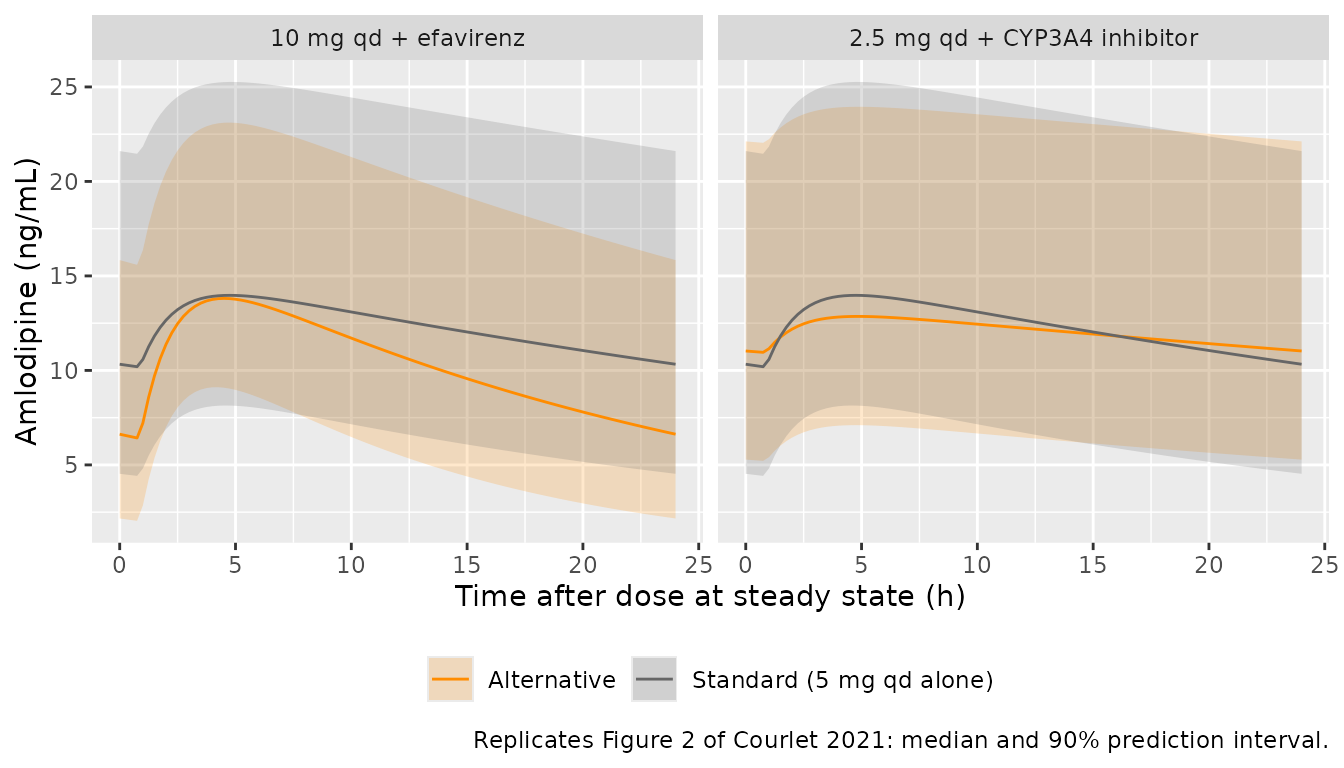

PKNCA validation

sim_nca <- sim |>
  dplyr::filter(!is.na(Cc)) |>
  dplyr::mutate(Cc = pmax(Cc, 0)) |>
  dplyr::select(id, time, Cc, treatment)

conc_obj <- PKNCA::PKNCAconc(sim_nca, Cc ~ time | treatment + id, concu = "ng/mL", timeu = "h")
dose_df <- events |>
  dplyr::filter(evid == 1) |>
  dplyr::select(id, time, amt, treatment)
dose_obj <- PKNCA::PKNCAdose(dose_df, amt ~ time | treatment + id, doseu = "mg")

intervals <- data.frame(start = 0, end = 24, cmax = TRUE, ctrough = TRUE, auclast = TRUE)
nca_res <- PKNCA::pk.nca(PKNCA::PKNCAdata(conc_obj, dose_obj, intervals = intervals))

published <- published_t3 |>
  dplyr::rename(treatment = regimen, auclast = auc024)

cmp <- nlmixr2lib::ncaComparisonTable(
  simulated = nca_res,
  reference = published,
  by = "treatment",
  units = c(cmax = "ng/mL", ctrough = "ng/mL", auclast = "ng*h/mL"),
  tolerance_pct = 20
)
knitr::kable(cmp, caption = "Simulated (median of the 200-subject quantile cohort) vs. Table 3 medians. * differs from reference by >20%.")

Simulated (median of the 200-subject quantile cohort) vs. Table 3 medians. * differs from reference by >20%.
NCA parameter	treatment	Reference	Simulated	% diff
Cmax (ng/mL)	5 mg qd alone	13.6	14	+2.7%
Cmax (ng/mL)	2.5 mg qd + CYP3A4 inhibitor	12.7	12.9	+1.2%
Cmax (ng/mL)	10 mg qd + efavirenz	13.7	13.8	+0.8%
AUClast (ng*h/mL)	5 mg qd alone	291	294	+1.1%
AUClast (ng*h/mL)	2.5 mg qd + CYP3A4 inhibitor	286	288	+0.9%
AUClast (ng*h/mL)	10 mg qd + efavirenz	242	245	+1.2%
Ctrough (ng/mL)	5 mg qd alone	10.2	10.3	+1.2%
Ctrough (ng/mL)	2.5 mg qd + CYP3A4 inhibitor	10.9	11	+1.2%
Ctrough (ng/mL)	10 mg qd + efavirenz	6.5	6.62	+1.9%

nca_df <- as.data.frame(nca_res) |>
  dplyr::filter(PPTESTCD %in% c("cmax", "ctrough", "auclast"))
stopifnot(nrow(nca_df) == 3L * 3L * n_per_arm)
sim_med <- nca_df |>
  dplyr::group_by(treatment, PPTESTCD) |>
  dplyr::summarise(med = median(PPORRES), .groups = "drop") |>
  tidyr::pivot_wider(names_from = PPTESTCD, values_from = med) |>
  dplyr::inner_join(published, by = "treatment", suffix = c("_sim", "_paper"))
stopifnot(nrow(sim_med) == 3L)
pct <- with(sim_med, 100 * c(
  cmax_sim / cmax_paper - 1,
  ctrough_sim / ctrough_paper - 1,
  auclast_sim / auclast_paper - 1
))
# The quantile cohort is deterministic, so this is not a Monte-Carlo gate;
# the remaining gap is the sampling noise in the paper's own 1000-subject
# medians plus trapezoidal AUC. Measured |difference| <= 3%. A
# mis-transcribed CL, V, ka, lag, covariate coefficient or unit moves at
# least one cell by well over 5%.
stopifnot(max(abs(pct)) < 5)

The simulated medians reproduce Table 3 to within 3% for all three regimens.

Prediction interval of AUC0-24

The width of the Table 3 AUC0-24 prediction interval depends only on the between-subject variance of CL/F, which makes it a check on the omega conversion (see Assumptions).

auc_pi <- nca_df |>
  dplyr::filter(PPTESTCD == "auclast") |>
  dplyr::group_by(treatment) |>
  dplyr::summarise(
    lo_sim = quantile(PPORRES, 0.025), hi_sim = quantile(PPORRES, 0.975),
    .groups = "drop"
  ) |>
  dplyr::inner_join(
    tibble::tribble(
      ~treatment,                     ~lo_paper, ~hi_paper,
      "5 mg qd alone",                129.3,     658.4,
      "2.5 mg qd + CYP3A4 inhibitor", 127.0,     646.8,
      "10 mg qd + efavirenz",         107.8,     548.7
    ),
    by = "treatment"
  )
stopifnot(nrow(auc_pi) == 3L)
auc_pi |>
  dplyr::mutate(dplyr::across(c(lo_sim, hi_sim), \(x) round(x, 1))) |>
  dplyr::rename(
    Regimen = treatment,
    "2.5th pct model" = lo_sim, "97.5th pct model" = hi_sim,
    "2.5th pct paper" = lo_paper, "97.5th pct paper" = hi_paper
  ) |>
  knitr::kable(caption = "AUC0-24 95% prediction interval (ng*h/mL), model versus Table 3.")

AUC0-24 95% prediction interval (ng*h/mL), model versus Table 3.
Regimen	2.5th pct model	97.5th pct model	2.5th pct paper	97.5th pct paper
10 mg qd + efavirenz	113.0	531.7	107.8	548.7
2.5 mg qd + CYP3A4 inhibitor	132.9	625.5	127.0	646.8
5 mg qd alone	135.6	638.0	129.3	658.4

# Measured: model bounds 3.1-4.8% inside the paper's (omega 0.403 here
# against the ~0.415 the paper's interval implies, plus the 200-point
# quantile grid). Reading the CV as omega = 0.42 or omega = 0.403 changes
# the bounds by about 3%; an omega mis-transcribed as a variance
# (0.42 -> omega 0.65) moves them by >40%.
stopifnot(
  max(abs(auc_pi$lo_sim / auc_pi$lo_paper - 1)) < 0.08,
  max(abs(auc_pi$hi_sim / auc_pi$hi_paper - 1)) < 0.08
)

Assumptions and deviations

Between-subject variability scale. Table 2 reports the BSV on CL/F as a CV of 42% without stating the conversion. The model encodes omega^2 = log(1 + 0.42^2) = 0.1625 (omega = 0.403). The Table 3 AUC0-24 prediction interval, which depends on this variance alone, implies an omega of about 0.415, between 0.403 and the alternative reading omega = 0.42; 1000 simulated subjects cannot separate the two (about 4% apart), and the packaged model’s interval sits 3-5% inside the published one.
Text versus equation for efavirenz. The Results text says the univariate efavirenz effect increased clearance by 40%, whereas Table 2 gives theta efavirenz = 1.40 in CL/F = 17.0 x ... x (1 + 1.40 x efavirenz), a 2.4-fold clearance. The equation is used: it alone reproduces the paper’s 59% lower AUC0-24 with efavirenz, the 0.83 AUC GMR of 10 mg with efavirenz in Table 3 and the 25% higher AUC with 15 mg (checked above).
Combined inhibitor and efavirenz. No subject received both; the model multiplies the two factors as the published equation does, which is an extrapolation outside the data.
Etravirine (18 samples) could not be separated from the ritonavir-boosted darunavir it was co-prescribed with and has no effect in the model; nevirapine was tested and not retained.
Base model. The Results also report the base-model estimates (ka 0.66 1/h, ALAG 0.86 h, V 980 L, CL 15.7 L/h, CV 61%); only the final model of Table 2 is packaged.
Figure 2 is reproduced without residual error, from the quantile cohort described under Virtual cohort; the paper does not state whether its prediction intervals include residual error.
No correction notice for this article was found in Europe PMC as of 2026-09-28.