Flucloxacillin (Jager 2020)
Source:vignettes/articles/Jager_2020_flucloxacillin.Rmd
Jager_2020_flucloxacillin.RmdModel and source
- Citation: Jager NGL, van Hest RM, Xie J, Wong G, Ulldemolins M, Bruggemann RJM, Lipman J, Roberts JA. Optimization of flucloxacillin dosing regimens in critically ill patients using population pharmacokinetic modelling of total and unbound concentrations. J Antimicrob Chemother. 2020;75(9):2641-2649. doi:10.1093/jac/dkaa187. PMCID PMC7443729. Binding equation from main-text Equation 3 (Supplementary Appendix 2 Equation 1); covariate equations from main-text Equations 4-5; parameter estimates from main-text Table 2 (final model column); unit conversion (flucloxacillin MW 453.9 g/mol) and residual-error form from Supplementary Appendix 2.
- Description: Two-compartment joint total/unbound population PK model for intravenous flucloxacillin in critically ill adults (Jager 2020). The disposition is carried on the UNBOUND concentration Cu = central/V1 with linear unbound clearance and linear intercompartmental exchange; the measured TOTAL plasma concentration is reconstructed as Cc = Cu + Bmax * Cu / (Kd + Cu), a single saturable binding site whose capacity Bmax rises with serum albumin. Total and unbound concentrations are BOTH observed endpoints, each with its own additive error on the log scale. Unbound clearance carries a power term on CKD-EPI eGFR. Inter-individual variability on CL and Bmax.
- Article: https://doi.org/10.1093/jac/dkaa187 (open access, PMC7443729)
- Supplementary data (Appendices 1-3, Figures S1-S3): available with the article at JAC Online.
Population
The model was built from 35 critically ill adults treated with intermittent intravenous flucloxacillin in the 30-bed ICU of the Royal Brisbane and Women’s Hospital, Australia. The data were pooled from two sources: a prospective PK study run in 2009 (10 hypoalbuminaemic patients, rich sampling of both total and unbound concentrations after at least 24 h of treatment) and a beta-lactam therapeutic-drug-monitoring programme run 2012-2014 (25 patients, mostly paired mid-interval and trough samples; unbound only in 19, total and unbound in 6). In total 79 total and 104 unbound concentrations were available (Methods; Results, Patients and samples).
Baseline characteristics (Table 1; median and IQR): 34% female, age 52 years (43-67), total body weight 95 kg (73-120), BMI 31 kg/m^2 (25-35), SOFA score 8 (5-13), CKD-EPI eGFR 96 (26-166), serum albumin 21 g/L (15-34); 11% were on renal replacement therapy. Every patient had albumin below 35 g/L. Doses ranged from 1 g q6h to 2 g q2h as 30-minute infusions. The observed protein binding was 63.4-97.2% (median 89.4%) and fell as total concentration rose (Figure 1), the signature of saturable binding.
The same information is recorded in the model’s
population metadata.
Model structure
The paper’s integrated model (Supplementary Appendix 2) runs the
two-compartment PK on the unbound drug: CL, V1, V2 and
Q are unbound-referenced, and the unbound central concentration is
Cu = central / V1. The total concentration is then the
unbound plus the bound concentration from a single saturable site
(Equation 3):
Ctotal = Cu + Bmax * Cu / (Kd + Cu)with the binding capacity rising with albumin and unbound clearance rising with renal function (Equations 4 and 5):
Bmax (mmol/L) = 0.469 * (Albumin / 20)^1.51
CL   (L/h)    = 55.4  * (eGFR / 90)^0.809
The fit was performed with every concentration converted to mmol/L (flucloxacillin MW 453.9 g/mol; Supplementary Appendix 2), so Bmax and Kd are kept in mmol/L exactly as printed and the model converts with the same molecular weight: Bmax 0.469 mmol/L is 212.9 mg/L and Kd 0.0441 mmol/L is 20.0 mg/L. Because albumin enters only the bound term, it moves total but not unbound concentrations – which is precisely what the paper reports from its own simulations (“Serum albumin concentrations did not affect unbound concentrations”, Figure 4b and d), and is verified below.
Source trace
| Model element | Value | Source |
|---|---|---|
| Two-compartment disposition on unbound drug | – | Results, PK analysis; Supplementary Appendix 2 (structural model) |
Ctotal = Cu + Bmax*Cu/(Kd+Cu) |
– | Equation 3; Supplementary Appendix 2 Equation 1 |
| Unit conversion, MW 453.9 g/mol | 453.9 | Supplementary Appendix 2 (structural model) |
lcl (CL at eGFR 90) |
55.4 L/h | Table 2, final model; Equation 5 |
lvc (V1) |
52.7 L | Table 2, final model |
lvp (V2) |
56.8 L | Table 2, final model |
lq (Q) |
67.2 L/h | Table 2, final model |
lbmax_pb (Bmax at albumin 20 g/L) |
0.469 mmol/L | Table 2, final model; Equation 4 |
lkd_pb (Kd) |
0.0441 mmol/L | Table 2, final model |
e_alb_bmax_pb |
1.51 | Table 2 covariates, albumin; Equation 4 |
e_crcl_cl |
0.809 | Table 2 covariates, eGFR; Equation 5 |
etalbmax_pb |
30.4 %CV -> 0.088384 | Table 2 BPV, final model |
etalcl |
71.6 %CV -> 0.413876 | Table 2 BPV, final model |
expSd (total) |
0.160 | Table 2 residual variability; Supplementary Appendix 2 (log-additive) |
expSd_Cu (unbound) |
0.222 | Table 2 residual variability; Supplementary Appendix 2 (log-additive) |
Binding isotherm
mod <- readModelDb("Jager_2020_flucloxacillin")
mod_typical <- rxode2::zeroRe(mod)
#> ℹ parameter labels from comments will be replaced by 'label()'

mw <- 453.9
bmax_mgL <- function(alb) 0.469 * (alb / 20)^1.51 * mw
kd_mgL <- 0.0441 * mw

binding <- tidyr::expand_grid(ALB = c(15, 21, 34), Cu = c(0.1, 1, 5, 10, 20, 30)) |>
  dplyr::mutate(
    Cb = bmax_mgL(ALB) * Cu / (kd_mgL + Cu),
    Ctot = Cu + Cb,
    pct_bound = 100 * Cb / Ctot
  )

binding |>
  dplyr::mutate(dplyr::across(c(Cb, Ctot, pct_bound), \(x) round(x, 1))) |>
  dplyr::rename(
    "Albumin (g/L)" = ALB,
    "Unbound (mg/L)" = Cu,
    "Bound (mg/L)" = Cb,
    "Total (mg/L)" = Ctot,
    "Protein binding (%)" = pct_bound
  ) |>
knitr::kable(caption = "Typical-value protein binding across the observed albumin IQR and unbound concentration range.")| Albumin (g/L) | Unbound (mg/L) | Bound (mg/L) | Total (mg/L) | Protein binding (%) |
|---|---|---|---|---|
| 15 | 0.1 | 0.7 | 0.8 | 87.3 |
| 15 | 1.0 | 6.6 | 7.6 | 86.8 |
| 15 | 5.0 | 27.6 | 32.6 | 84.6 |
| 15 | 10.0 | 45.9 | 55.9 | 82.1 |
| 15 | 20.0 | 68.9 | 88.9 | 77.5 |
| 15 | 30.0 | 82.7 | 112.7 | 73.4 |
| 21 | 0.1 | 1.1 | 1.2 | 91.9 |
| 21 | 1.0 | 10.9 | 11.9 | 91.6 |
| 21 | 5.0 | 45.8 | 50.8 | 90.2 |
| 21 | 10.0 | 76.3 | 86.3 | 88.4 |
| 21 | 20.0 | 114.5 | 134.5 | 85.1 |
| 21 | 30.0 | 137.4 | 167.4 | 82.1 |
| 34 | 0.1 | 2.4 | 2.5 | 95.9 |
| 34 | 1.0 | 22.6 | 23.6 | 95.8 |
| 34 | 5.0 | 94.8 | 99.8 | 95.0 |
| 34 | 10.0 | 158.0 | 168.0 | 94.0 |
| 34 | 20.0 | 237.1 | 257.1 | 92.2 |
| 34 | 30.0 | 284.5 | 314.5 | 90.5 |
The observed range of protein binding was 63.4-97.2% over unbound concentrations of 0.1-30 mg/L and albumin of roughly 15-34 g/L (Results, Protein binding). The typical-value isotherm must fall inside that envelope over the same domain, must fall with concentration at fixed albumin (Figure 1) and must rise with albumin at fixed concentration (Figure 2).
# Deterministic; no random draws involved.
stopifnot(
  all(binding$pct_bound > 63.4 & binding$pct_bound < 97.2),
  all(tapply(binding$pct_bound, binding$ALB, \(x) all(diff(x) < 0))),
  all(tapply(binding$pct_bound, binding$Cu, \(x) all(diff(x) > 0)))
)
The model’s own Cc must reproduce the same isotherm. At
an unbound concentration equal to Kd the bound concentration is exactly
Bmax / 2.
# Run a typical patient to steady state and check Cc against the closed-form
# isotherm evaluated at the model's own Cu.
ev_iso <- rxode2::et(amt = 2000, dur = 0.5, cmt = "central", ii = 4, until = 48) |>
  rxode2::et(seq(0, 48, by = 0.25)) |>
  as.data.frame() |>
  dplyr::mutate(CRCL = 96, ALB = 21, dvid = ifelse(evid == 0, 1L, NA_integer_))

sim_iso <- rxode2::rxSolve(mod_typical, ev_iso, omega = NA, sigma = NA,
                           returnType = "data.frame") |>
  dplyr::mutate(Cc_closed = Cu + bmax_mgL(21) * Cu / (kd_mgL + Cu))

stopifnot(max(abs(sim_iso$Cc - sim_iso$Cc_closed) / sim_iso$Cc_closed, na.rm = TRUE) < 1e-8)
Replicating Figure 4: effect of eGFR and albumin
Figure 4 shows typical-patient profiles over the first 24 h of 1 g q6h and 2 g q4h, for eGFR at the 10th and 90th percentiles (33 and 153) crossed with albumin at the 10th and 90th percentiles (15 and 30 g/L).
fig4_grid <- tidyr::expand_grid(
  regimen = c("1 g q6h", "2 g q4h"),
  CRCL = c(33, 153),
  ALB = c(15, 30)
) |>
  dplyr::mutate(id = dplyr::row_number())

make_fig4 <- function(regimen, CRCL, ALB, id) {
  amt <- if (regimen == "1 g q6h") 1000 else 2000
  tau <- if (regimen == "1 g q6h") 6 else 4
  rxode2::et(amt = amt, dur = 0.5, cmt = "central", ii = tau, addl = 24 / tau - 1) |>
    rxode2::et(seq(0, 24, by = 0.1)) |>
    as.data.frame() |>
    dplyr::mutate(id = id, CRCL = CRCL, ALB = ALB, regimen = regimen,
                  dvid = ifelse(evid == 0, 1L, NA_integer_))
}

ev_fig4 <- dplyr::bind_rows(Map(make_fig4, fig4_grid$regimen, fig4_grid$CRCL, fig4_grid$ALB, fig4_grid$id))

sim_fig4 <- rxode2::rxSolve(mod_typical, ev_fig4, omega = NA, sigma = NA,
                            keep = c("regimen", "CRCL", "ALB"),
                            returnType = "data.frame") |>
  dplyr::mutate(scenario = paste0("eGFR ", CRCL, ", Alb ", ALB))

sim_fig4 |>
  dplyr::select(time, regimen, scenario, Total = Cc, Unbound = Cu) |>
  tidyr::pivot_longer(c(Total, Unbound), names_to = "analyte", values_to = "conc") |>
  ggplot(aes(time, conc, colour = scenario)) +
  geom_line() +
  facet_grid(analyte ~ regimen, scales = "free_y") +
  scale_x_continuous(breaks = seq(0, 24, by = 4)) +
  labs(x = "Time (h)", y = "Flucloxacillin (mg/L)", colour = NULL,
       caption = "Replicates Figure 4 of Jager 2020 (typical patient, first 24 h).")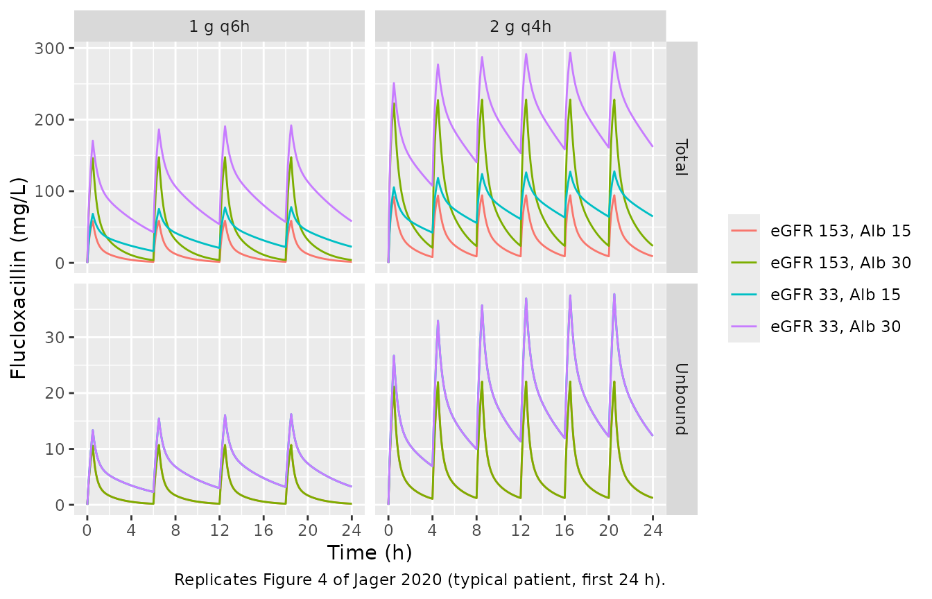
chk4 <- sim_fig4 |>
  dplyr::select(time, regimen, CRCL, ALB, Cc, Cu) |>
  tidyr::pivot_wider(names_from = ALB, values_from = c(Cc, Cu))

stopifnot(
  # Albumin does not change unbound concentrations (Results, Figure 4b/d).
  max(abs(chk4$Cu_15 - chk4$Cu_30)) < 1e-10,
  # ...but a higher albumin raises total concentrations (Figure 4a/c).
  all(chk4$Cc_30[chk4$time > 0] > chk4$Cc_15[chk4$time > 0])
)

# Higher eGFR lowers the 24-h trough, total and unbound, for both regimens.
tr24 <- sim_fig4 |> dplyr::filter(time == 24)
stopifnot(all(
  tapply(seq_len(nrow(tr24)), paste(tr24$regimen, tr24$ALB), function(i) {
    d <- tr24[i, ]
    d$Cu[d$CRCL == 153] < d$Cu[d$CRCL == 33] && d$Cc[d$CRCL == 153] < d$Cc[d$CRCL == 33]
  })
))
PKNCA validation
Unbound flucloxacillin is linear, so over a steady-state interval its AUC must equal Dose / CL and its terminal half-life must equal ln 2 / beta, where beta is the slower root of the two-compartment disposition. The check runs at the three eGFR values the paper used for target attainment (33, 96 and 153) on 2 g q4h.
egfr_levels <- c(33, 96, 153)

make_ss_arm <- function(egfr, id) {
  rxode2::et(amt = 2000, dur = 0.5, cmt = "central", ii = 4, until = 96) |>
    rxode2::et(c(0, seq(96, 100, by = 0.05))) |>
    as.data.frame() |>
    dplyr::mutate(id = id, CRCL = egfr, ALB = 21,
                  dvid = ifelse(evid == 0, 2L, NA_integer_),
                  treatment = paste0("eGFR ", egfr))
}

ev_nca <- dplyr::bind_rows(Map(make_ss_arm, egfr_levels, seq_along(egfr_levels)))

sim_nca <- rxode2::rxSolve(mod_typical, ev_nca, omega = NA, sigma = NA,
                           keep = c("treatment", "CRCL"),
                           returnType = "data.frame")

conc_df <- sim_nca |>
  dplyr::filter(!is.na(Cu)) |>
  dplyr::select(id, time, Cu, treatment)

dose_df <- ev_nca |>
  dplyr::filter(evid == 1) |>
  dplyr::select(id, time, amt, treatment)

conc_obj <- PKNCA::PKNCAconc(conc_df, Cu ~ time | treatment + id)
dose_obj <- PKNCA::PKNCAdose(dose_df, amt ~ time | treatment + id)

intervals <- data.frame(start = 96, end = 100, auclast = TRUE, cmax = TRUE,
                        half.life = TRUE)

nca_res <- PKNCA::pk.nca(PKNCA::PKNCAdata(conc_obj, dose_obj, intervals = intervals))
beta_of <- function(cl, vc = 52.7, vp = 56.8, q = 67.2) {
  k10 <- cl / vc; k12 <- q / vc; k21 <- q / vp
  s <- k10 + k12 + k21
  (s - sqrt(s^2 - 4 * k10 * k21)) / 2
}

closed <- tibble::tibble(CRCL = egfr_levels) |>
  dplyr::mutate(
    treatment = paste0("eGFR ", CRCL),
    cl = 55.4 * (CRCL / 90)^0.809,
    auc_closed = 2000 / cl,
    hl_closed = log(2) / beta_of(cl)
  )

nca_wide <- as.data.frame(nca_res) |>
  dplyr::filter(PPTESTCD %in% c("auclast", "cmax", "half.life")) |>
  dplyr::select(treatment, PPTESTCD, PPORRES) |>
  tidyr::pivot_wider(names_from = PPTESTCD, values_from = PPORRES) |>
  dplyr::left_join(closed, by = "treatment") |>
  dplyr::mutate(
    auc_pct = 100 * (auclast - auc_closed) / auc_closed,
    hl_pct = 100 * (half.life - hl_closed) / hl_closed
  ) |>
  dplyr::arrange(CRCL)

nca_wide |>
  dplyr::select(treatment, cmax, auclast, auc_closed, auc_pct, half.life, hl_closed, hl_pct) |>
  dplyr::mutate(dplyr::across(where(is.numeric), \(x) round(x, 2))) |>
  dplyr::rename(
    "Renal stratum" = treatment,
    "Cmax,u (mg/L)" = cmax,
    "PKNCA AUCtau,u (mg*h/L)" = auclast,
    "Dose/CL (mg*h/L)" = auc_closed,
    "AUC difference (%)" = auc_pct,
    "PKNCA t1/2 (h)" = half.life,
    "ln2/beta (h)" = hl_closed,
    "t1/2 difference (%)" = hl_pct
  ) |>
knitr::kable(caption = "Unbound NCA over a steady-state 2 g q4h interval against the model's closed-form identities.")| Renal stratum | Cmax,u (mg/L) | PKNCA AUCtau,u (mg*h/L) | Dose/CL (mg*h/L) | AUC difference (%) | PKNCA t1/2 (h) | ln2/beta (h) | t1/2 difference (%) |
|---|---|---|---|---|---|---|---|
| eGFR 33 | 37.93 | 81.28 | 81.29 | 0.00 | 3.36 | 3.42 | -1.58 |
| eGFR 96 | 25.61 | 34.26 | 34.26 | -0.02 | 1.64 | 1.67 | -1.48 |
| eGFR 153 | 22.06 | 23.49 | 23.50 | -0.03 | 1.27 | 1.28 | -1.23 |
# Solve against its own closed form: pure numerical error, so a tight bound
# is correct. The half-life bound allows for PKNCA fitting the terminal slope
# over a 4-h interval in which the distribution phase has not fully decayed.
stopifnot(
  all(abs(nca_wide$auc_pct) < 1),
  all(abs(nca_wide$hl_pct) < 10)
)
The paper does not tabulate NCA parameters, so the comparison above is against the model’s own closed form; the published target-attainment results below are the external check.
Replicating Figure 5: probability of target attainment
The paper simulated four regimens at eGFR 33, 96 and 153 for a patient with otherwise median characteristics, and computed the probability that the unbound concentration stays above the MIC for the whole dosing interval at t = 24 h (Figure 5). Unbound concentration falls monotonically after each infusion ends, so this is the unbound concentration at 24 h, the trough of the last dose of the first day. The cohort here is 200 virtual patients per regimen-and-eGFR arm (the paper used 1000).
rxode2::rxSetSeed(20200416)
n_per_arm <- 200

pta_grid <- tidyr::expand_grid(
  regimen = c("1 g q6h", "1 g q4h", "2 g q6h", "2 g q4h"),
  CRCL = c(33, 96, 153)
) |>
  dplyr::mutate(arm = dplyr::row_number())

make_pta_arm <- function(regimen, CRCL, arm) {
  amt <- if (startsWith(regimen, "1 g")) 1000 else 2000
  tau <- if (endsWith(regimen, "q6h")) 6 else 4
  rxode2::et(amt = amt, dur = 0.5, cmt = "central", ii = tau, addl = 24 / tau - 1) |>
    rxode2::et(24) |>
    rxode2::et(id = seq_len(n_per_arm) + (arm - 1) * n_per_arm) |>
    as.data.frame() |>
    dplyr::mutate(CRCL = CRCL, ALB = 21, regimen = regimen,
                  dvid = ifelse(evid == 0, 2L, NA_integer_))
}

ev_pta <- dplyr::bind_rows(Map(make_pta_arm, pta_grid$regimen, pta_grid$CRCL, pta_grid$arm))

sim_pta <- rxode2::rxSolve(mod, ev_pta, sigma = NA,
                           keep = c("regimen", "CRCL"),
                           returnType = "data.frame")
#> ℹ parameter labels from comments will be replaced by 'label()'

mics <- c(0.125, 0.25, 0.5, 1, 2)

pta <- sim_pta |>
  dplyr::filter(time == 24) |>
  tidyr::crossing(MIC = mics) |>
  dplyr::group_by(regimen, CRCL, MIC) |>
  dplyr::summarise(PTA = 100 * mean(Cu >= MIC), .groups = "drop")

ggplot(pta, aes(MIC, PTA, colour = factor(CRCL))) +
  geom_line() +
  geom_point() +
  scale_x_log10(breaks = mics) +
  facet_wrap(~regimen) +
  labs(x = "MIC (mg/L)", y = "PTA, 100% fT>MIC (%)", colour = "eGFR",
       caption = "Replicates Figure 5 of Jager 2020 (200 virtual patients per arm).")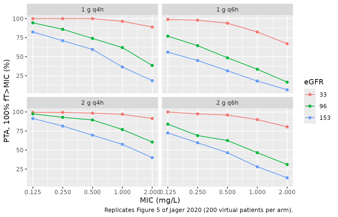
published <- tibble::tribble(
  ~regimen,  ~CRCL, ~MIC, ~PTA_paper,
  "1 g q6h",  33,   0.5,  91,
  "2 g q4h",  96,   0.5,  87,
  "2 g q4h", 153,   0.5,  71,
  "2 g q4h",  33,   2,    95,
  "2 g q4h",  96,   2,    57,
  "2 g q4h", 153,   2,    36
)

pta_cmp <- published |>
  dplyr::left_join(pta, by = c("regimen", "CRCL", "MIC")) |>
  dplyr::mutate(diff = PTA - PTA_paper)

pta_cmp |>
  dplyr::mutate(PTA = round(PTA, 1), diff = round(diff, 1)) |>
  dplyr::rename(
    "Regimen" = regimen, "eGFR" = CRCL, "MIC (mg/L)" = MIC,
    "Published PTA (%)" = PTA_paper, "Simulated PTA (%)" = PTA,
    "Difference (points)" = diff
  ) |>
knitr::kable(caption = "Every probability of target attainment the paper prints in its Results, against this simulation.")| Regimen | eGFR | MIC (mg/L) | Published PTA (%) | Simulated PTA (%) | Difference (points) |
|---|---|---|---|---|---|
| 1 g q6h | 33 | 0.5 | 91 | 94.0 | 3.0 |
| 2 g q4h | 96 | 0.5 | 87 | 89.5 | 2.5 |
| 2 g q4h | 153 | 0.5 | 71 | 69.5 | -1.5 |
| 2 g q4h | 33 | 2.0 | 95 | 91.5 | -3.5 |
| 2 g q4h | 96 | 2.0 | 57 | 60.5 | 3.5 |
| 2 g q4h | 153 | 2.0 | 36 | 40.0 | 4.0 |
The six printed PTAs are the Results-section values (Abstract and Results, Monte Carlo dosing simulations). With 200 patients per arm the binomial standard error of a PTA is at most 3.5 points; the bound below is about four standard errors, wide enough to hold for whatever cohort a given rxode2 build draws but far tighter than the shift a mis-transcribed clearance, exponent or variance would cause.
stopifnot(
  all(abs(pta_cmp$diff) < 15),
  # Paper, Results: MIC 0.25 mg/L on 2 g q4h gives >90% up to eGFR 96 but
  # not at eGFR 153. Asserted with margin on the robust side only.
  pta$PTA[pta$regimen == "2 g q4h" & pta$CRCL == 33 & pta$MIC == 0.25] > 90,
  pta$PTA[pta$regimen == "2 g q4h" & pta$CRCL == 153 & pta$MIC == 0.25] < 95
)
Assumptions and deviations
- Between-patient variability scale. Table 2 reports BPV as %CV for exponential random effects without stating the conversion. The model uses the log-normal identity omega^2 = log(CV^2 + 1) (0.0884 for Bmax, 0.4139 for CL). The alternative reading omega^2 = CV^2 (0.0924 and 0.5127) was also simulated during extraction: both reproduce the published target-attainment percentages within a few points, so the paper cannot discriminate between them.
-
Residual error. Supplementary Appendix 2 describes
an additive error on log-transformed data with SDs 0.16 (total) and 0.22
(unbound), and translates them to 17-18% and 24-25%, which are exp(SD) -
1. Table 2 labels the same numbers “proportional error”. They are
encoded as
lnorm()SDs. -
eGFR units. The paper writes eGFR in mL/min, but it
is the CKD-EPI creatinine equation, whose native output is mL/min/1.73
m^2, and no de-normalization is described. The column is the
BSA-normalized canonical
CRCL; supply CKD-EPI values as reported by the laboratory. - Albumin extrapolation. All patients had albumin below 35 g/L; the authors caution against using the model above that.
-
Target-attainment simulation. The paper does not
state whether residual error was included in its Monte Carlo
simulations; the replication here uses between-patient variability only
(
sigma = NA), which reproduces the published values. The albumin value is irrelevant to unbound PTA. - Renal replacement therapy. Four patients were on RRT; RRT was not a retained covariate, so the model has no dialysis term.
- Errata. No erratum or correction was found for this article (Crossref and journal landing page, checked 2026-09-27).