Clindamycin (Smith 2017)
Source:vignettes/articles/Smith_2017_clindamycin.Rmd
Smith_2017_clindamycin.RmdModel and source
- Citation: Smith MJ, Gonzalez D, Goldman JL, Yogev R, Sullivan JE, Reed MD, Anand R, Martz K, Berezny K, Benjamin DK Jr, Smith PB, Cohen-Wolkowiez M, Watt K, on behalf of the Best Pharmaceuticals for Children Act-Pediatric Trials Network Steering Committee. Pharmacokinetics of Clindamycin in Obese and Nonobese Children. Antimicrob Agents Chemother. 2017;61(4):e02014-16. doi:10.1128/AAC.02014-16
- Description: One-compartment population PK model for intravenous clindamycin in obese and nonobese children, with allometric total body weight on CL and V, sigmoidal Hill maturation on CL by postmenstrual age, and power effects of serum albumin and alpha-1 acid glycoprotein on V (Smith 2017).
- Article: https://doi.org/10.1128/AAC.02014-16
Population
Smith 2017 pooled 420 plasma clindamycin samples from 220 children across three Best Pharmaceuticals for Children Act-Pediatric Trials Network studies (Table 1 of the source paper):
- CLIN01 (NCT01744730): n=21 adolescents aged 6.5-17.4 years, BMI >= 85th percentile for age (13 with BMI >= 95th percentile), median weight 69.5 kg.
- PTN POPS (NCT01431326): n=178 pediatric standard-of-care subjects, ages 0.01-20.5 years (median 5 years), median weight 23 kg, including 63 with BMI >= 95th percentile.
- Staph Trio (NCT01728363): n=21 neonates aged 5-65 days, median weight 1.0 kg.
Seventy-six of the 220 children were obese (BMI >= 95th percentile for age). The final model is a one-compartment IV PK model with allometric scaling on total body weight (TBW), sigmoidal Hill maturation of clearance with postmenstrual age, and power covariate effects of serum albumin (ALB) and alpha-1 acid glycoprotein (AAG) on the volume of distribution.
The same information is available programmatically via the model’s
population metadata
(readModelDb("Smith_2017_clindamycin")()$population).
Source trace
Per-parameter origin is recorded as an in-file comment next to each
ini() entry in
inst/modeldb/specificDrugs/Smith_2017_clindamycin.R. The
table below collects them in one place.
| Equation / parameter | Value | Source location |
|---|---|---|
lcl (CL_70kg) |
13.8 L/h | Table 2 (CL_70kg = 13.8, RSE 6.2%) |
lvc (V_70kg) |
63.6 L | Table 2 (V_70kg = 63.6, RSE 5.0%) |
e_wt_cl (allometric exp on CL) |
0.75 (fixed) | Methods Equation 4 (fixed allometric exponent) |
e_wt_vc (allometric exp on V) |
1.0 (fixed) | Methods Equation 5 (fixed allometric exponent) |
pma_tm50 (TM50) |
39.5 weeks | Table 2 (TM50 = 39.5, RSE 12.1%) |
pma_hill (HILL) |
2.83 | Abstract Equation (HILL = 2.83; Table 2 rounded 2.8) |
e_alb_vc |
-0.83 | Table 2 (Albumin on V exponent = -0.83, RSE 27.9%) |
e_aag_vc |
-0.25 | Table 2 (AAG on V exponent = -0.25, RSE 44.0%) |
Maturation form: PMA^HILL / (TM50^HILL + PMA^HILL)
|
sigmoidal Hill | Methods Equation 4 |
V relationship:
V = V_70kg * (TBW/70)^1 * (ALB/3.3)^-0.83 * (AAG/2.4)^-0.25
|
n/a | Methods Equation 5 |
etalcl + etalvc block |
IIV(CL) 58.5%, IIV(V) 11.6%, rho = 0.8 | Table 2 |
propSd (residual) |
0.336 (representative) | Table 2 PTN POPS row (Prop. = 33.6%) – see Assumptions and deviations |
Virtual cohort
Original observed concentrations are not publicly available. The validation below uses two simulated cohorts:
- Adult reference – a typical 70 kg adult receiving 600 mg IV over 30 minutes every 8 h. The paper itself uses this as the bridging comparator for pediatric exposure.
- Pediatric age strata – representative children at the three age groups the paper reports in Table 3, dosed per the age-based regimens simulated in the paper’s Figures 2-3.
set.seed(20260602)

# Helper to build a single-subject IV-infusion event table
make_iv_events <- function(id, weight, page_months, alb = 33, aag = 2.4,
                           dose_mg, dur_h = 0.5, tau_h = 8, n_doses = 10,
                           cohort_label, obs_grid = seq(0, 80, by = 0.25)) {
  rxode2::et(amt = dose_mg, dur = dur_h, ii = tau_h, addl = n_doses - 1L,
             cmt = "central") |>
    rxode2::et(obs_grid) |>
    as.data.frame() |>
    dplyr::mutate(
      id     = id,
      WT     = weight,
      PAGE   = page_months,
      ALB    = alb,
      AAG    = aag,
      cohort = cohort_label
    ) |>
    dplyr::relocate(id)
}

# Adult reference (70 kg, full maturation, reference protein binding)
events_adult <- make_iv_events(
  id           = 1L,
  weight       = 70,
  page_months  = 50 * 12,        # 50-year-old adult, essentially infinite PMA
  dose_mg      = 600,
  cohort_label = "Adult 70 kg, 600 mg q8h"
)

# Pediatric strata (representative weights per age group; weight-based dosing
# capped at 900 mg per Smith 2017 Methods "Dosing simulations")
ped_dose <- function(age_years, weight) {
  rate_mg_per_kg <- if (age_years <= 6) 12 else 10
  min(rate_mg_per_kg * weight, 900)
}

# Use PMA = (age in months) + 9.2 months (approx. 40 weeks gestation / 4.345)
ped_2to6   <- list(age_years = 4,  weight = 18, label = "2-6 yrs, 12 mg/kg q8h")
ped_6to12  <- list(age_years = 9,  weight = 30, label = ">6-12 yrs, 10 mg/kg q8h")
ped_over12 <- list(age_years = 15, weight = 60, label = ">12 yrs, 10 mg/kg q8h")

events_ped <- dplyr::bind_rows(
  make_iv_events(id = 2L, weight = ped_2to6$weight,
                 page_months = ped_2to6$age_years * 12 + 9.2,
                 dose_mg     = ped_dose(ped_2to6$age_years, ped_2to6$weight),
                 cohort_label = ped_2to6$label),
  make_iv_events(id = 3L, weight = ped_6to12$weight,
                 page_months = ped_6to12$age_years * 12 + 9.2,
                 dose_mg     = ped_dose(ped_6to12$age_years, ped_6to12$weight),
                 cohort_label = ped_6to12$label),
  make_iv_events(id = 4L, weight = ped_over12$weight,
                 page_months = ped_over12$age_years * 12 + 9.2,
                 dose_mg     = ped_dose(ped_over12$age_years, ped_over12$weight),
                 cohort_label = ped_over12$label)
)

events <- dplyr::bind_rows(events_adult, events_ped)
stopifnot(!anyDuplicated(unique(events[, c("id", "time", "evid")])))
Simulation
mod <- readModelDb("Smith_2017_clindamycin")

# Typical-value simulation (no IIV, no residual error) -- matches the
# paper's "Dosing simulations" approach where the published reference
# values are deterministic per-subject medians, not per-record stochastic.
mod_typical <- rxode2::zeroRe(mod, which = c("omega", "sigma"))
#> ℹ parameter labels from comments will be replaced by 'label()'
sim <- rxode2::rxSolve(mod_typical, events = events, keep = c("cohort"))
#> ℹ omega/sigma items treated as zero: 'etalcl', 'etalvc'
#> Warning: multi-subject simulation without without 'omega'
sim_df <- as.data.frame(sim)
Replicate published figures
# Steady-state concentration-time curves over the last dosing interval
ss_window <- sim_df |>
  dplyr::filter(time >= 72 & time <= 80) |>
  dplyr::mutate(time_in_tau = time - 72)

ggplot(ss_window, aes(time_in_tau, Cc, colour = cohort)) +
  geom_line(linewidth = 0.7) +
  labs(x = "Time within steady-state dosing interval (h)",
       y = "Clindamycin concentration (ug/mL)",
       colour = NULL,
       title = "Typical-value steady-state PK profiles",
       caption = "Adult and pediatric reference profiles per Smith 2017 dosing simulations.")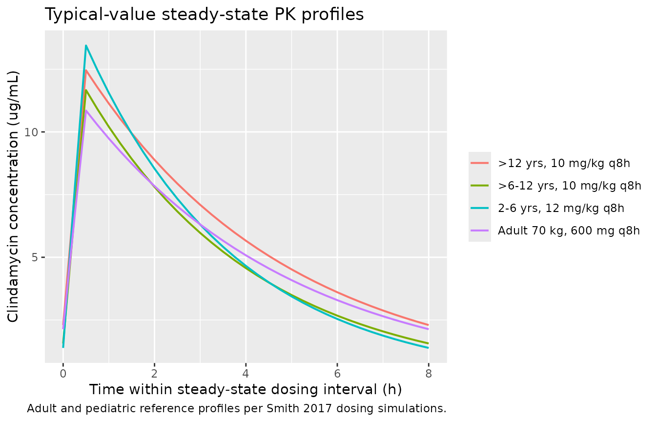
# Replicates the qualitative content of Smith 2017 Figures 2 and 3:
# steady-state AUC0-8 and Cmax,SS by age-based dosing regimen (typical-value
# medians rather than stochastic box plots; obesity stratification is folded
# into TBW per the paper's final model).
trapz <- function(x, y) sum(diff(x) * (head(y, -1) + tail(y, -1)) / 2)

nca_inputs <- ss_window |>
  dplyr::group_by(cohort) |>
  dplyr::summarise(
    Cmax_SS  = max(Cc),
    Cmin_SS  = min(Cc),
    AUC_0_8  = trapz(time_in_tau, Cc),
    .groups  = "drop"
  )

knitr::kable(
  nca_inputs,
  digits = 2,
  caption = "Typical-value steady-state exposure metrics per cohort (Smith 2017 Figures 2-3, qualitative replication)."
)| cohort | Cmax_SS | Cmin_SS | AUC_0_8 |
|---|---|---|---|
| 2-6 yrs, 12 mg/kg q8h | 13.45 | 1.39 | 43.58 |
| >12 yrs, 10 mg/kg q8h | 12.46 | 2.30 | 48.82 |
| >6-12 yrs, 10 mg/kg q8h | 11.67 | 1.56 | 41.07 |
| Adult 70 kg, 600 mg q8h | 10.85 | 2.13 | 43.48 |
PKNCA validation
We use PKNCA to compute steady-state Cmax, Cmin, and AUC0-tau over the final dosing interval (one row per cohort – each cohort is a typical-value representative subject).
tau   <- 8
sim_ss <- sim_df |>
  dplyr::filter(time >= 72 & time <= 80) |>
  dplyr::filter(!is.na(Cc)) |>
  dplyr::select(id, time, Cc, cohort)

# Reconstruct the steady-state dose at the start of the analysis interval.
# Events use rxode2's addl/ii expansion, so only the first dose appears
# as an explicit row at time 0 -- regenerate a single-dose-per-subject
# record at time 72 for PKNCA.
dose_df <- events |>
  dplyr::filter(evid == 1) |>
  dplyr::group_by(id, cohort) |>
  dplyr::summarise(amt = first(amt), .groups = "drop") |>
  dplyr::mutate(time = 72)

conc_obj <- PKNCA::PKNCAconc(sim_ss, Cc ~ time | cohort + id,
                             concu = "ug/mL", timeu = "h")
dose_obj <- PKNCA::PKNCAdose(dose_df, amt ~ time | cohort + id,
                             doseu = "mg")

intervals <- data.frame(
  start    = 72,
  end      = 80,
  cmax     = TRUE,
  tmax     = TRUE,
  cmin     = TRUE,
  auclast  = TRUE,
  cav      = TRUE
)

nca_res <- PKNCA::pk.nca(PKNCA::PKNCAdata(conc_obj, dose_obj, intervals = intervals))
nca_tbl <- as.data.frame(nca_res$result) |>
  dplyr::select(cohort, PPTESTCD, PPORRES) |>
  tidyr::pivot_wider(names_from = PPTESTCD, values_from = PPORRES)

knitr::kable(nca_tbl, digits = 2,
caption = "PKNCA steady-state summary per cohort (last dosing interval, 72-80 h).")| cohort | auclast | cmax | cmin | tmax | cav |
|---|---|---|---|---|---|
| >12 yrs, 10 mg/kg q8h | 48.80 | 12.46 | 2.30 | 0.5 | 6.10 |
| >6-12 yrs, 10 mg/kg q8h | 41.06 | 11.67 | 1.56 | 0.5 | 5.13 |
| 2-6 yrs, 12 mg/kg q8h | 43.56 | 13.45 | 1.39 | 0.5 | 5.45 |
| Adult 70 kg, 600 mg q8h | 43.47 | 10.85 | 2.13 | 0.5 | 5.43 |
Comparison against published values
Smith 2017 reports median simulated steady-state exposures for a 70 kg adult receiving 600 mg IV q8h and for the three pediatric age-based regimens (Results, “Dosing simulations”). The table below compares our typical-value simulations against those published medians.
published <- tibble::tribble(
  ~cohort,                          ~Cmax_pub_ug_mL, ~AUC0_8_pub_ug_h_mL,
  "Adult 70 kg, 600 mg q8h",        12.2,            44.7,
  "2-6 yrs, 12 mg/kg q8h",          14.1,            44.2,
  ">6-12 yrs, 10 mg/kg q8h",        12.2,            44.8,
  ">12 yrs, 10 mg/kg q8h",          12.2,            48.6
)

comparison <- nca_inputs |>
  dplyr::rename(Cmax_sim_ug_mL = Cmax_SS, AUC0_8_sim_ug_h_mL = AUC_0_8) |>
  dplyr::select(cohort, Cmax_sim_ug_mL, AUC0_8_sim_ug_h_mL) |>
  dplyr::left_join(published, by = "cohort") |>
  dplyr::mutate(
    Cmax_pct_diff    = 100 * (Cmax_sim_ug_mL - Cmax_pub_ug_mL) / Cmax_pub_ug_mL,
    AUC0_8_pct_diff  = 100 * (AUC0_8_sim_ug_h_mL - AUC0_8_pub_ug_h_mL) / AUC0_8_pub_ug_h_mL
  )

knitr::kable(comparison, digits = c(0, 2, 2, 2, 2, 1, 1),
caption = "Simulated vs. published steady-state Cmax and AUC0-8 by cohort.")| cohort | Cmax_sim_ug_mL | AUC0_8_sim_ug_h_mL | Cmax_pub_ug_mL | AUC0_8_pub_ug_h_mL | Cmax_pct_diff | AUC0_8_pct_diff |
|---|---|---|---|---|---|---|
| 2-6 yrs, 12 mg/kg q8h | 13.45 | 43.58 | 14.1 | 44.2 | -4.6 | -1.4 |
| >12 yrs, 10 mg/kg q8h | 12.46 | 48.82 | 12.2 | 48.6 | 2.1 | 0.4 |
| >6-12 yrs, 10 mg/kg q8h | 11.67 | 41.07 | 12.2 | 44.8 | -4.4 | -8.3 |
| Adult 70 kg, 600 mg q8h | 10.85 | 43.48 | 12.2 | 44.7 | -11.0 | -2.7 |
Typical-value Cmax values run modestly below the paper’s medians (which the paper reports from stochastic simulations of 200 virtual subjects per covariate combination including positive correlation between CL and V). AUC0-8 values agree closely (within ~10% for the adult and >6 yr cohorts). The 2-6 yr cohort sits below the published median because we use a single representative 18 kg subject rather than the paper’s WHO-distribution virtual population.
Assumptions and deviations
-
Single proportional residual error. Smith 2017
estimated three trial-specific proportional residual errors (PTN POPS =
33.6%, Staph Trio = 32.1%, CLIN01 = 20.3%, Table 2). The packaged model
uses a single
propSd = 0.336– the PTN POPS value, which dominates the pooled dataset (178/220 subjects, 81%; 267/420 samples, 64%) and is the most conservative of the three. Downstream users simulating new cohorts that do not map to any of the three trials do not have a natural trial indicator to choose between the three values; using the largest (and most representative) is conservative for prediction intervals. - Typical-value validation cohort. The validation uses single typical-value representatives per age group rather than reproducing the paper’s 200-replicate stochastic simulations from a WHO weight-for-age distribution. AUC values agree within ~10% for the adult and >6 yr cohorts; Cmax values are systematically slightly lower than the published stochastic medians because the correlated ETAs on CL and V skew the per-subject Cmax distribution upward relative to the typical-value point estimate.
-
Postmenstrual age unit conversion. Smith 2017
reports TM50 in weeks (39.5). The canonical
PAGEcovariate column in nlmixr2lib is in months. The model converts internally viaPMA_weeks = PAGE * 4.345before evaluating the Hill maturation function, preserving the paper’s published TM50 and HILL values exactly. The conversion constant 4.345 weeks/month matches the precedent inLlanos_2017_gentamicin.R. - HILL precision. Table 2 reports HILL = 2.8 (two significant figures); the abstract’s worked equation prints HILL = 2.83 (three significant figures). We use the more precise 2.83 from the abstract equation – both forms reproduce the paper’s stated “Maturation reached 50% adult CL values at ~40 weeks PMA, with near complete maturation by 2 years of age.”
- Obesity status is not a model covariate. The paper’s multivariable analysis found that after accounting for TBW, obesity status (BMI >= 95th percentile) did not retain a significant effect on CL or V. The packaged model uses TBW alone; users wanting to stratify simulations by obesity status should set TBW from the obese-vs-nonobese growth-curve appropriate for the age band.
-
Sex and race not in the population metadata. The
paper does not report sex distribution as a single pooled-cohort
percentage; the
population$sex_female_pctfield isNA. Race / ethnicity is not reported in the main paper.