Polymyxin B and mucin against Acinetobacter baumannii (Lacroix 2025)
Source:vignettes/articles/Lacroix_2025_polymyxinB_mucin.Rmd
Lacroix_2025_polymyxinB_mucin.RmdModels and source
This paper contributes two model files, one per bacterial strain.
- Citation: Lacroix M, Moreau J, Zampaloni C, Bissantz C, Mirfendereski H, Shirvani H, Marchand S, Couet W, Chauzy A. (2025). In vitro pharmacokinetic/pharmacodynamic modeling of the effect of mucin on polymyxin B activity against Acinetobacter baumannii. Antimicrobial Agents and Chemotherapy 69(5):e01535-24. doi:10.1128/aac.01535-24. Structural model: supplemental text (AAC01535-24-S0002) Eqs S1-S6 and supplemental Fig. S2 (left panel, AB121-D0), which prints the final kill-rate and covariate equations. Unbound-fraction model: main-text Eq 1. Parameter estimates: main-text Table 1 (fu model) and Table 3, columns ‘AB121-D0 without mucin’ and ‘AB121-D0 with mucin’.
- Article: Antimicrob Agents Chemother 69(5):e01535-24
| Model file | Strain | Kill function | Mucin acts on |
|---|---|---|---|
Lacroix_2025_polymyxinB_AB121D0 |
AB121-D0, isolated before colistin treatment | Emax (no Hill term) |
Emax_R (1.4-fold increase) |
Lacroix_2025_polymyxinB_AB122D12 |
AB122-D12, isolated 12 days after colistin treatment | Sigmoidal Emax |
Knet (halved) and EC50 (5-fold rise) |
mod121 <- rxode2::rxode2(nlmixr2lib::readModelDb("Lacroix_2025_polymyxinB_AB121D0"))
#> ℹ parameter labels from comments will be replaced by 'label()'
mod122 <- rxode2::rxode2(nlmixr2lib::readModelDb("Lacroix_2025_polymyxinB_AB122D12"))
#> ℹ parameter labels from comments will be replaced by 'label()'
Population and experimental system
Two multidrug-resistant Acinetobacter baumannii clinical
isolates recovered from the same patient, before
(AB121-D0) and 12 days after (AB122-D12) colistin treatment. AB122-D12
carries a 10-amino-acid insertion in pmrB
(p.21_22insCILIFSVILG) that confers polymyxin B (PMB) resistance.
Static time-kill (TK) experiments were run in cation-adjusted
Mueller-Hinton broth (CAMHB) with or without 1% (w/v) porcine-stomach
mucin, at 35 degrees C with shaking, starting from roughly 1e6 CFU/mL
and sampled at 0, 1, 3, 6, 10, 24 and 30 h. The limit of quantification
was 400 CFU/mL (2.6 log10 CFU/mL). PMB was assumed stable over the
experiment, so the applied concentration is time-invariant and is
carried in these models as the covariate CONC_PMB_MGL
rather than as a PK compartment. The second covariate,
MUCIN_PRESENT, is the binary medium indicator.
str(mod121$meta$population)
#> List of 8
#>  $ species     : chr "in vitro (Acinetobacter baumannii AB121-D0)"
#>  $ n_subjects  : int NA
#>  $ n_studies   : int 1
#>  $ organism    : chr "A. baumannii AB121-D0, a multidrug-resistant clinical isolate recovered from a patient before colistin treatmen"| __truncated__
#>  $ model_system: chr "Static time-kill (TK) experiments in glass tubes, 35 degrees C with shaking at 150-170 rpm, in commercial CAMHB"| __truncated__
#>  $ dose_range  : chr "Total PMB 0.5 to 128 mg/L (plus a drug-free growth control); with 1% mucin these correspond to unbound PMB conc"| __truncated__
#>  $ lloq        : chr "400 CFU/mL, i.e. 2.6 log10 CFU/mL (CLSI); observations below it were handled by Beal's M3 method during estimation."
#>  $ notes       : chr "Estimated in NONMEM 7.4.2 with the LAPLACIAN algorithm on log10-transformed bacterial counts; uncertainty by sa"| __truncated__
Model structure
Both strains use the same hetero-resistance (S/R) skeleton: a
susceptible subpopulation bact_s and a resistant
subpopulation bact_r growing logistically with a shared
apparent net rate constant Knet toward the carrying
capacity BMAX, each depleted by its own
concentration-dependent kill rate (supplemental Eqs S1-S4):
d(bact_s)/dt = Knet * (1 - (bact_s + bact_r)/BMAX) * bact_s - Kill_S * bact_s
d(bact_r)/dt = Knet * (1 - (bact_s + bact_r)/BMAX) * bact_r - Kill_R * bact_r
The inoculum is split by MUT, the log10
proportion of the initial population that is
resistant.
Mucin binds PMB, so the killing effect is driven by the
unbound concentration Cu = C_T * fu, where
fu follows a saturable sigmoidal Emax function of the
total concentration (main-text Eq 1). Without mucin
there is nothing to bind PMB, so fu is 1. Beyond binding,
mucin also shifts the PD parameters through the categorical selector of
main-text Eq 4, P = theta_1 * (1 - Mucin) + theta_2 * Mucin
– acting on Emax_R for AB121-D0 and on Knet
and EC50 for AB122-D12 (supplemental Fig. S2).
Source trace
| Quantity | Source location |
|---|---|
| Logistic growth, both subpopulations (Eqs S1-S2) | Supplemental text S0002, “Bacterial growth sub-model” |
| Kill terms subtracted from each subpopulation (Eqs S3-S4) | Supplemental text S0002, “Drug effect sub-model” |
| AB121-D0 kill rates: Emax, no Hill (Eqs S5-S6) | Supplemental text S0002; Fig. S2 left panel |
| AB122-D12 kill rates: sigmoidal Emax (Eqs S7-S8) | Supplemental text S0002; Fig. S2 right panel |
Unbound fraction fu vs total PMB (Eq 1) |
Main text, “PMB binding to mucin” |
| Between-experiment additive etas on the Eq 1 parameters (Eqs 2-3) | Main text, “Pharmacodynamic modeling” |
| Categorical mucin selector (Eq 4) | Main text, “Pharmacodynamic modeling” |
Mucin placement: Emax_R (AB121-D0); Knet +
EC50 (AB122-D12) |
Fig. S2 caption; Results, “TK experiment and PK/PD modeling” |
E0 0.061, Imax 0.56, IC50
114.37, epsilon 1.97 (+ variances) |
Table 1 (pooled data set) |
INOC, BMAX, MUT,
Knet, Emax_S, Emax_R,
EC50, gamma, sigma
|
Table 3 |
| MIC and unbound-MIC values | Table 2 |
| Regrowth concentration thresholds | Results, “TK experiment and PK/PD modeling” |
| Inoculum, sampling times, LOQ | Materials and Methods, “TK experiments” |
Validation
This is a mechanistic in-vitro bacterial-dynamics model, not a plasma
PK model: the drug concentration is a static experimental input and the
observation is a log10 viable count. Non-compartmental analysis is
therefore not the right check, and PKNCA is not used. Instead the model
is validated against four published answer keys – the tabulated
fu values, the structural growth identities, the unbound
MICs, and the reported regrowth-concentration thresholds – plus the
paper’s directional claims about how mucin changes PMB activity.
# Typical-value simulation: zeroRe() drops the fixed-variance fu etas.
simTk <- function(model, conc, mucin, tmax = 30, by = 0.25) {
  ev <- rxode2::et(seq(0, tmax, by = by))
  d <- as.data.frame(ev)
  d$id <- 1L
  d$CONC_PMB_MGL <- conc
  d$MUCIN_PRESENT <- mucin
  out <- rxode2::rxSolve(rxode2::zeroRe(model), d,
                         omega = NA, sigma = NA, returnType = "data.frame")
  stopifnot(nrow(out) == nrow(d))
  out
}

# Unbound fraction from Eq 1, using the packaged ini() values.
ini121 <- as.data.frame(mod121$iniDf)
thetaOf <- function(df, nm) df$est[df$name == nm & is.na(df$neta1)]
fuEq1 <- function(ct) {
  e0 <- thetaOf(ini121, "fu_e0")
  imax <- thetaOf(ini121, "fu_imax")
  ic50 <- thetaOf(ini121, "fu_ic50")
  eps <- thetaOf(ini121, "fu_hill")
  e0 + imax * ct^eps / (ic50^eps + ct^eps)
}
1. Unbound-fraction sub-model against Table S2
Table S2 of the supplement tabulates fu simulated from
Eq 1 with the pooled parameter set across four orders of magnitude of
total PMB. Reproducing that column exercises every parameter of the
binding sub-model at once.
fuCheck <-
  data.frame(
    total_mgL = c(0.5, 1, 2, 4, 8, 10, 50, 100, 500, 1000, 5000, 10000),
    published_pct = c(6.1, 6.1, 6.1, 6.1, 6.4, 6.5, 15.2, 30.4, 59.2, 61.3, 62.1, 62.1)
  ) |>
  dplyr::mutate(
    model_pct = round(100 * fuEq1(total_mgL), 2),
    difference = round(model_pct - published_pct, 2),
    unbound_mgL = signif(total_mgL * fuEq1(total_mgL), 3)
  )

fuCheck |>
  dplyr::rename(
    "Total PMB (mg/L)" = total_mgL,
    "fu published (%)" = published_pct,
    "fu model (%)" = model_pct,
    "Difference (pp)" = difference,
    "Unbound PMB (mg/L)" = unbound_mgL
  ) |>
knitr::kable(caption = "Replicates Table S2 of Lacroix 2025 (pooled-data column).")| Total PMB (mg/L) | fu published (%) | fu model (%) | Difference (pp) | Unbound PMB (mg/L) |
|---|---|---|---|---|
| 5e-01 | 6.1 | 6.10 | 0.00 | 3.05e-02 |
| 1e+00 | 6.1 | 6.10 | 0.00 | 6.10e-02 |
| 2e+00 | 6.1 | 6.12 | 0.02 | 1.22e-01 |
| 4e+00 | 6.1 | 6.18 | 0.08 | 2.47e-01 |
| 8e+00 | 6.4 | 6.40 | 0.00 | 5.12e-01 |
| 1e+01 | 6.5 | 6.56 | 0.06 | 6.56e-01 |
| 5e+01 | 15.2 | 15.27 | 0.07 | 7.64e+00 |
| 1e+02 | 30.4 | 30.42 | 0.02 | 3.04e+01 |
| 5e+02 | 59.2 | 59.20 | 0.00 | 2.96e+02 |
| 1e+03 | 61.3 | 61.33 | 0.03 | 6.13e+02 |
| 5e+03 | 62.1 | 62.07 | -0.03 | 3.10e+03 |
| 1e+04 | 62.1 | 62.09 | -0.01 | 6.21e+03 |
# Every tabulated value must be reproduced to within 0.1 percentage points.
stopifnot(max(abs(fuCheck$difference)) < 0.1)
Replicating Figure 1 – fu rises from about 6% to a 62%
plateau, with the sigmoid centred on IC50 = 114 mg/L:
fuCurve <- data.frame(total = 10^seq(log10(0.5), log10(10000), length.out = 200))
fuCurve$fu <- 100 * fuEq1(fuCurve$total)

ggplot2::ggplot(fuCurve, ggplot2::aes(total, fu)) +
  ggplot2::geom_line(linewidth = 1) +
  ggplot2::geom_point(
    data = fuCheck,
    ggplot2::aes(total_mgL, published_pct), colour = "firebrick", size = 2
  ) +
  ggplot2::scale_x_log10() +
  ggplot2::labs(
    x = "Total PMB concentration (mg/L)",
    y = "PMB unbound fraction (%)",
    caption = "Line: Eq 1 from the packaged model. Points: Table S2 published values."
  ) +
  ggplot2::theme_bw()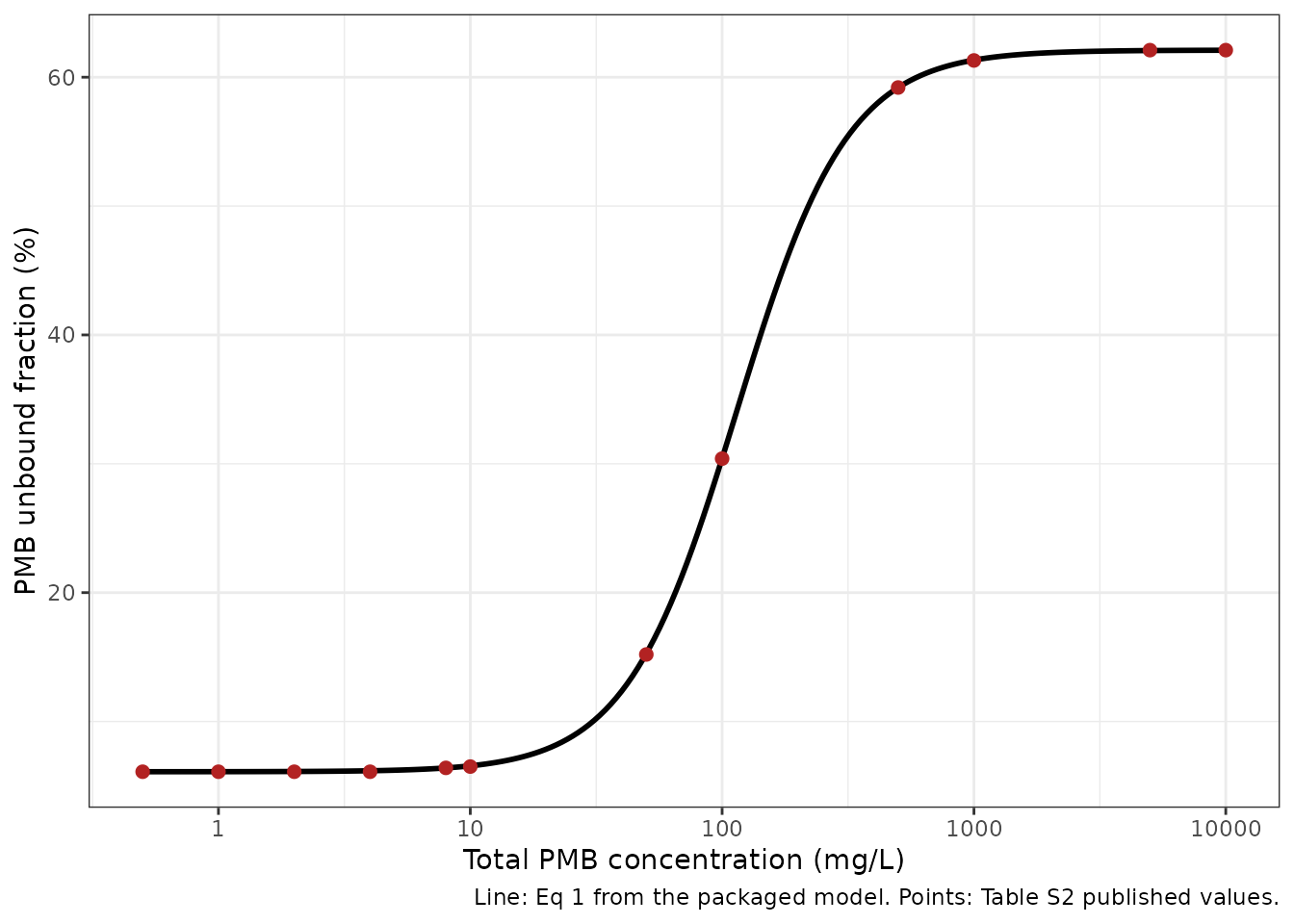
Replicates Figure 1 of Lacroix 2025.
2. Structural growth identities
With no drug the kill terms vanish and both ODEs collapse to pure
logistic growth. Two identities must then hold exactly: the count at
time zero is INOC, and the plateau is BMAX.
Both are read back from the packaged ini() rather than
hard-coded.
growthCheck <- lapply(
  list(`AB121-D0` = mod121, `AB122-D12` = mod122),
  function(m) {
    ini <- as.data.frame(m$iniDf)
    r <- simTk(m, conc = 0, mucin = 0, tmax = 48)
    data.frame(
      t0_model = round(r$log_cfu[1], 3),
      t0_INOC = thetaOf(ini, "log10_inoc"),
      plateau_model = round(max(r$log_cfu), 3),
      plateau_BMAX = thetaOf(ini, "log10_cfumax")
    )
  }
) |>
  dplyr::bind_rows(.id = "Strain")

growthCheck |>
  dplyr::rename(
    "log10 CFU/mL at t=0" = t0_model,
    "INOC (Table 3)" = t0_INOC,
    "log10 CFU/mL plateau" = plateau_model,
    "BMAX (Table 3)" = plateau_BMAX
  ) |>
knitr::kable(caption = "Growth-control identities against Table 3.")| Strain | log10 CFU/mL at t=0 | INOC (Table 3) | log10 CFU/mL plateau | BMAX (Table 3) |
|---|---|---|---|---|
| AB121-D0 | 6.00 | 6.00 | 8.47 | 8.47 |
| AB122-D12 | 5.45 | 5.45 | 8.14 | 8.14 |
3. Unbound MICs against Table 2
Table 2 reports MICs in CAMHB and in CAMHB + 1% mucin, and converts
the latter to unbound MICs by multiplying by fu.
Recomputing that conversion with the packaged Eq 1 parameters is an
independent check on the binding sub-model at exactly the two
concentrations the paper used.
micCheck <-
  data.frame(
    strain = c("AB121-D0", "AB122-D12"),
    mic_camhb = c(1, 32),
    mic_mucin = c(64, 1024),
    published_micu = c(13, 628)
  ) |>
  dplyr::mutate(
    model_micu = round(mic_mucin * fuEq1(mic_mucin)),
    published_ratio = round(published_micu / mic_camhb),
    model_ratio = round(model_micu / mic_camhb)
  )

micCheck |>
  dplyr::rename(
    "Strain" = strain,
    "MIC CAMHB (mg/L)" = mic_camhb,
    "MIC +1% mucin (mg/L)" = mic_mucin,
    "MICu published (mg/L)" = published_micu,
    "MICu model (mg/L)" = model_micu,
    "MICu ratio published" = published_ratio,
    "MICu ratio model" = model_ratio
  ) |>
knitr::kable(caption = "Replicates Table 2 of Lacroix 2025.")| Strain | MIC CAMHB (mg/L) | MIC +1% mucin (mg/L) | MICu published (mg/L) | MICu model (mg/L) | MICu ratio published | MICu ratio model |
|---|---|---|---|---|---|---|
| AB121-D0 | 1 | 64 | 13 | 13 | 13 | 13 |
| AB122-D12 | 32 | 1024 | 628 | 628 | 20 | 20 |
4. Time-kill profiles
Replicating the shape of Figures S1 and 2 – an initial CFU decay followed by regrowth driven by the resistant subpopulation, at the concentrations actually tested for each strain.
concGrid <- list(
  `AB121-D0` = list(model = mod121, conc = c(0, 0.5, 1, 4, 8, 16, 128)),
  `AB122-D12` = list(model = mod122, conc = c(0, 8, 32, 64, 128, 256, 512))
)

tkProfiles <- lapply(names(concGrid), function(s) {
  g <- concGrid[[s]]
  lapply(g$conc, function(cc) {
    simTk(g$model, conc = cc, mucin = 0) |>
      dplyr::mutate(Strain = s, conc = cc)
  }) |> dplyr::bind_rows()
}) |> dplyr::bind_rows()

ggplot2::ggplot(
  tkProfiles,
  ggplot2::aes(time, log_cfu, colour = factor(conc), group = factor(conc))
) +
  ggplot2::geom_line(linewidth = 0.8) +
  ggplot2::geom_hline(yintercept = 2.6, linetype = "dashed", colour = "grey40") +
  ggplot2::facet_wrap(~Strain) +
  ggplot2::labs(
    x = "Time (h)", y = "log10 CFU/mL", colour = "Total PMB\n(mg/L)",
    caption = "CAMHB without mucin (fu = 1). Dashed line: 2.6 log10 CFU/mL limit of quantification."
  ) +
  ggplot2::theme_bw()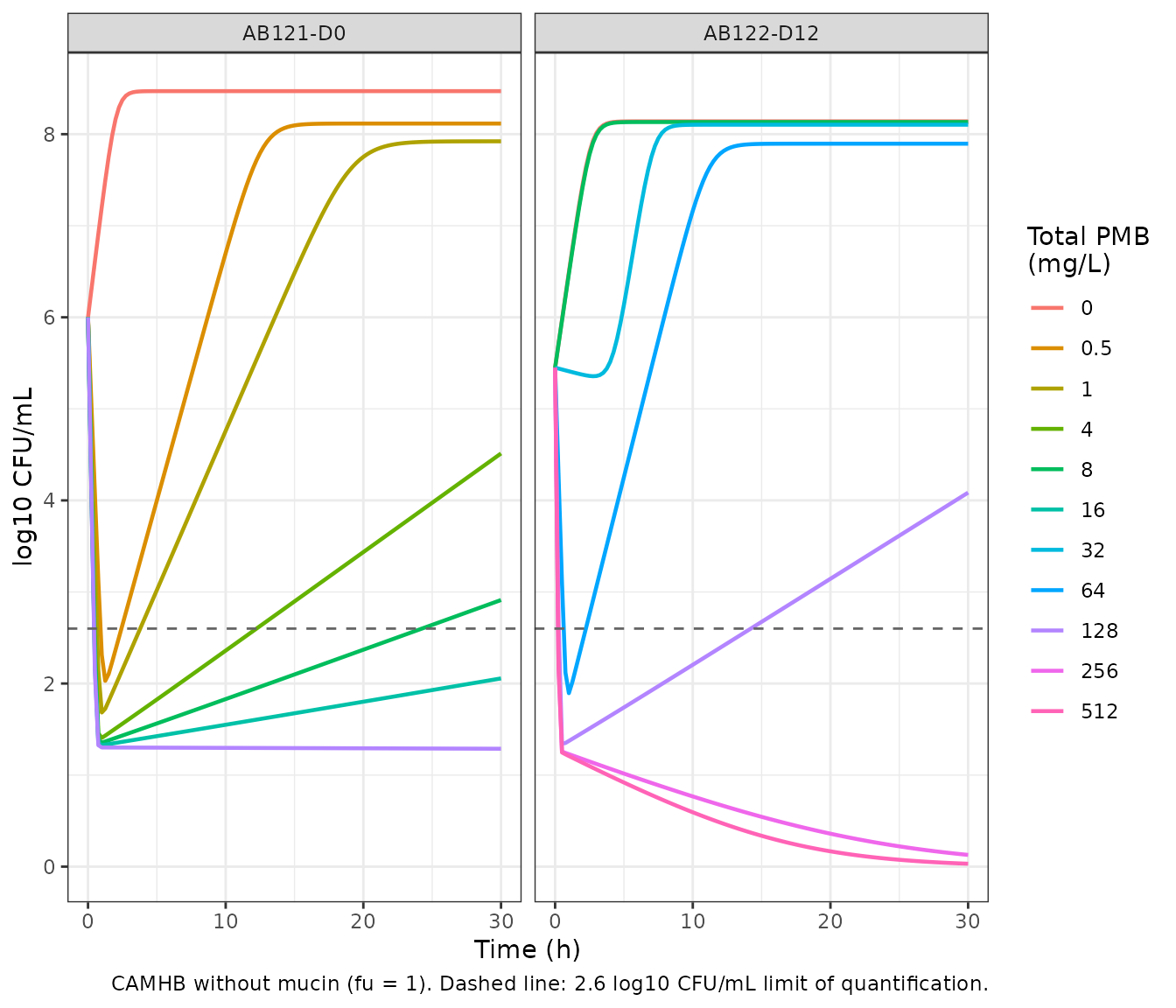
Replicates the CAMHB panels of Figure S1 / Figure 2 of Lacroix 2025.
5. Regrowth thresholds against the published Results
The Results state that in CAMHB regrowth followed the initial decay
“for PMB concentrations up to 8 mg/L for AB121-D0 and 128 mg/L for
AB122-D12”. That threshold is a whole-model answer key: it depends
jointly on INOC, MUT, BMAX,
Knet, both Emax values, EC50 and
(for AB122-D12) gamma. Regrowth is scored as a 30-h count
at least 1 log10 above the nadir.
regrew <- function(model, conc) {
  r <- simTk(model, conc = conc, mucin = 0)
  utils::tail(r$log_cfu, 1) > min(r$log_cfu) + 1
}

thresholdCheck <-
  dplyr::bind_rows(
    data.frame(
      Strain = "AB121-D0", conc = c(0.5, 1, 2, 4, 8, 16, 32, 64, 128),
      regrowth = vapply(c(0.5, 1, 2, 4, 8, 16, 32, 64, 128),
                        function(x) regrew(mod121, x), logical(1))
    ),
    data.frame(
      Strain = "AB122-D12", conc = c(8, 16, 32, 64, 128, 256, 512),
      regrowth = vapply(c(8, 16, 32, 64, 128, 256, 512),
                        function(x) regrew(mod122, x), logical(1))
    )
  )

highestRegrowth <- thresholdCheck |>
  dplyr::filter(regrowth) |>
  dplyr::group_by(Strain) |>
  dplyr::summarise(model_mgL = max(conc), .groups = "drop") |>
  dplyr::mutate(published_mgL = c(8, 128)[match(Strain, c("AB121-D0", "AB122-D12"))])

highestRegrowth |>
  dplyr::rename(
    "Highest regrowth conc., model (mg/L)" = model_mgL,
    "Highest regrowth conc., published (mg/L)" = published_mgL
  ) |>
knitr::kable(caption = "Replicates the regrowth thresholds reported in Results.")| Strain | Highest regrowth conc., model (mg/L) | Highest regrowth conc., published (mg/L) |
|---|---|---|
| AB121-D0 | 8 | 8 |
| AB122-D12 | 128 | 128 |
6. Direction of the mucin effect at matched unbound concentration
The paper’s central finding is that mucin changes PMB activity beyond binding, and in opposite directions for the two strains: activity increases for AB121-D0 and decreases for AB122-D12. The correct comparison holds the unbound concentration fixed, so any difference is attributable to the residual mucin effect rather than to binding.
The concentrations below are chosen to sit in each strain’s
pharmacologically active range. Far below EC50 the
comparison carries no information: neither arm is meaningfully killed,
both populations reach the carrying capacity, and the two 30-h counts
coincide. For AB122-D12, whose EC50 is 73.3 mg/L without
mucin and 384 mg/L with it, that means the informative totals are the
upper part of the tested range.
matchedPair <- function(model, totalWithMucin) {
  cu <- totalWithMucin * fuEq1(totalWithMucin)
  data.frame(
    total_mucin_mgL = totalWithMucin,
    unbound_mgL = signif(cu, 3),
    with_mucin = round(utils::tail(simTk(model, totalWithMucin, 1)$log_cfu, 1), 2),
    without_mucin = round(utils::tail(simTk(model, cu, 0)$log_cfu, 1), 2)
  )
}

mucinDirection <-
  dplyr::bind_rows(
    lapply(c(4, 8, 128), function(x) matchedPair(mod121, x)) |>
      dplyr::bind_rows() |> dplyr::mutate(Strain = "AB121-D0"),
    lapply(c(128, 256, 512), function(x) matchedPair(mod122, x)) |>
      dplyr::bind_rows() |> dplyr::mutate(Strain = "AB122-D12")
  ) |>
  dplyr::mutate(delta = round(with_mucin - without_mucin, 2)) |>
  dplyr::select(Strain, dplyr::everything())

mucinDirection |>
  dplyr::rename(
    "Total PMB + mucin (mg/L)" = total_mucin_mgL,
    "Matched unbound PMB (mg/L)" = unbound_mgL,
    "30-h log10 CFU with mucin" = with_mucin,
    "30-h log10 CFU without mucin" = without_mucin,
    "Difference (log10)" = delta
  ) |>
knitr::kable(caption = "Mucin effect at matched unbound PMB concentration.")| Strain | Total PMB + mucin (mg/L) | Matched unbound PMB (mg/L) | 30-h log10 CFU with mucin | 30-h log10 CFU without mucin | Difference (log10) |
|---|---|---|---|---|---|
| AB121-D0 | 4 | 0.247 | 8.15 | 8.26 | -0.11 |
| AB121-D0 | 8 | 0.512 | 7.82 | 8.11 | -0.29 |
| AB121-D0 | 128 | 47.600 | 0.00 | 1.47 | -1.47 |
| AB122-D12 | 128 | 47.600 | 8.12 | 8.03 | 0.09 |
| AB122-D12 | 256 | 135.000 | 8.10 | 3.44 | 4.66 |
| AB122-D12 | 512 | 304.000 | 7.29 | 0.07 | 7.22 |
# AB121-D0: mucin INCREASES activity, so the 30-h count is lower.
# AB122-D12: mucin DECREASES activity, so the 30-h count is higher.
stopifnot(
  all(mucinDirection$delta[mucinDirection$Strain == "AB121-D0"] < 0),
  all(mucinDirection$delta[mucinDirection$Strain == "AB122-D12"] > 0)
)
The paper further reports that for AB122-D12 “no PMB concentration in the range tested (up to 304 mg/L) was able to prevent bacterial regrowth in the presence of mucin”, whereas the same unbound concentration without mucin is bactericidal. The highest tested total concentration, 512 mg/L, corresponds to 304 mg/L unbound:
topRow <- mucinDirection |>
  dplyr::filter(Strain == "AB122-D12", total_mucin_mgL == 512)

stopifnot(
  # With mucin, the population has regrown to near the carrying capacity.
  topRow$with_mucin > 7,
  # Without mucin, at the same unbound concentration, it is eradicated.
  topRow$without_mucin < 2.6
)
topRow$unbound_mgL
#> [1] 304
7. Mucin arms with the between-experiment random effects
The published model’s only random effects are additive etas on the four Eq 1 parameters, with variances fixed to the Table 1 estimation variances. They propagate binding uncertainty into each simulated TK experiment, so they matter only in the mucin arms. Simulating 100 experiments per concentration (well under the 200-per-arm cap) shows the resulting spread in the mucin time-kill profiles.
set.seed(20250326)
nExp <- 100
mucinConc <- c(0.5, 4, 8, 128)

stochastic <- lapply(mucinConc, function(cc) {
  ev <- rxode2::et(seq(0, 30, by = 0.5)) |> rxode2::et(id = seq_len(nExp))
  d <- as.data.frame(ev)
  d$CONC_PMB_MGL <- cc
  d$MUCIN_PRESENT <- 1
  rxode2::rxSolve(mod121, d, sigma = NA, returnType = "data.frame") |>
    dplyr::mutate(conc = cc)
}) |> dplyr::bind_rows()

# rxSolve silently drops subjects on failure; assert the count survived.
stopifnot(
  dplyr::n_distinct(stochastic$id) == nExp,
  all(is.finite(stochastic$log_cfu))
)

stochastic |>
  dplyr::group_by(conc, time) |>
  dplyr::summarise(
    lo = quantile(log_cfu, 0.05), md = median(log_cfu), hi = quantile(log_cfu, 0.95),
    .groups = "drop"
  ) |>
  ggplot2::ggplot(ggplot2::aes(time, md)) +
  ggplot2::geom_ribbon(ggplot2::aes(ymin = lo, ymax = hi), alpha = 0.25,
                       fill = "turquoise4") +
  ggplot2::geom_line(linewidth = 0.8, colour = "turquoise4") +
  ggplot2::geom_hline(yintercept = 2.6, linetype = "dashed", colour = "grey40") +
  ggplot2::facet_wrap(~conc, labeller = ggplot2::label_both) +
  ggplot2::labs(
    x = "Time (h)", y = "log10 CFU/mL",
    caption = paste(
      "AB121-D0 in CAMHB + 1% mucin. Median and 90% interval over", nExp,
      "simulated experiments; spread comes from the fixed-variance fu etas."
    )
  ) +
  ggplot2::theme_bw()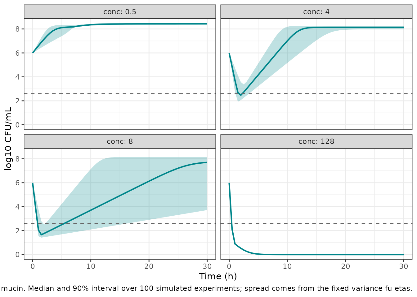
Between-experiment variability from the fixed-variance fu etas (AB121-D0, with mucin).
Assumptions and deviations
-
Inoculum split.
MUTis reported as the log10 proportion of resistant bacteria in the initial inoculum. These files split the inoculum mass-conservatively –bact_r(0) = 10^INOC * 10^MUTandbact_s(0) = 10^INOC * (1 - 10^MUT). The paper does not print the initial conditions explicitly. The alternative reading, in which the susceptible compartment starts at the full10^INOCwithout subtracting the resistant fraction, differs by under 0.002% of the inoculum for both strains (10^-4.72and10^-4.19) and is invisible on a log10 CFU scale. -
fuoutside the mucin arm. The paper states that MICs measured without mucin correspond directly to unbound MICs, so these files setfu = 1whenMUCIN_PRESENTis 0. Eq 1 is applied only in the mucin arm; it was estimated from mucin-containing broth and has no meaning without mucin. -
Observation floor.
log_cfuis computed aslog10(bact_s + bact_r + 1). The 1 CFU/mL floor keeps the observation finite when PMB sterilises the tube; it is 2.6 log10 below the 400 CFU/mL limit of quantification and so cannot affect any comparison against reported data. The same device is used by the siblingCheah_2016_polymyxin_*models. - Below-quantification data. The published fit used Beal’s M3 method for observations below the 400 CFU/mL LOQ. M3 is an estimation-time likelihood device with no simulation-time counterpart, so it is not represented here; simulated profiles are shown unfiltered and the LOQ is drawn as a reference line.
-
Additive etas can in principle go negative. The Eq
1 random effects are additive on natural-scale parameters with variances
fixed to the Table 1 estimation variances, exactly as published. The
epsiloneta (variance 0.252 on a mean of 1.97) and theE0eta (variance 0.0004 on a mean of 0.061) sit roughly 4 and 3 standard deviations above zero respectively, so a negative draw is possible though rare. This is a faithful transcription of the published parameterisation rather than a modelling choice; usezeroRe()for deterministic work, as the typical-value sections above do. -
Residual error is not applied in the figures.
log_cfuis the individual prediction; the additivesigmafrom Table 3 (0.35 and 0.33 log10 CFU/mL) is declared in the model but the plotted profiles usesigma = NAso that the structural behaviour is visible. - No IIV on the PD parameters. The published model has none – the only random effects are the four fixed-variance binding etas. No etas were invented.
-
Resistance mechanisms are not modelled.
Whole-genome sequencing found
pmrABC(AB121-D0) andlpxACD(AB122-D12) mutations in only some regrowth replicates, and the authors note explicitly that the S/R structure is a simplification that does not map onto the observed genotypes. The model is phenomenological in that respect. -
Non-ASCII characters (Greek letters, en-dashes)
from the source are transliterated throughout (
epsilon,gamma,-).
Errata
No erratum or corrigendum was found for this article at the time of extraction (checked against the journal landing page and PubMed).
The main-text Table 3 as typeset splits the gamma and
sigma rows across the strain columns in a way that is easy
to misread; the parameter assignments used here were confirmed against
the paper’s own arithmetic – Emax_R 2.84 to 3.90 is the
stated 1.4-fold mucin increase, Knet 2.42 to 1.34 the
stated twofold decrease, and EC50 73.3 to 384 the stated
fivefold increase.