Naproxen WOMAC pain time-course MBMA (Boucher 2018)
Source:vignettes/articles/Boucher_2018_naproxen_mbma.Rmd
Boucher_2018_naproxen_mbma.RmdModel and source
- Citation: Boucher M, Bennetts M. The Many Flavors of Model-Based Meta-Analysis: Part II: Modeling Summary Level Longitudinal Responses. CPT Pharmacometrics Syst Pharmacol. 2018 May;7(5):288-297. doi:10.1002/psp4.12299.
- Description: MBMA. Model-based meta-analysis longitudinal time-course Emax model for the Western Ontario and McMaster Universities (WOMAC) pain score (0-10 scale) in adults with osteoarthritis, fitted to study-arm-mean data from 18 randomized double-blind placebo-controlled trials of naproxen vs placebo (12 flare designs, 6 non-flare). The WOMAC pain response over time follows a three-parameter Emax model in time: pain = E0 + Emax * time / (ET50 + time), where ET50 is the time to half-maximal effect. Flare design shifts both baseline E0 and Emax; naproxen treatment shifts Emax and shortens ET50 (faster onset: ET50 0.21 week vs placebo 0.69 week). Between-study variability is carried as study-arm-level random effects on E0 (SD 0.62) and Emax (SD 0.74); the residual describes study-arm-mean variability weighted by each arm’s observed standard error (sigma fixed to 1). Suitable simulation scope is study-arm-mean WOMAC pain time-course, NOT individual-patient pain scores. Parameter values are the NONMEM column of Table 2 (the same model was fit in NONMEM, BUGS, and R with closely agreeing estimates).
- Article: https://doi.org/10.1002/psp4.12299
This is the worked example from Part II of Boucher and Bennetts’ model-based meta-analysis (MBMA) tutorial. It is a longitudinal time-course model: the Western Ontario and McMaster Universities (WOMAC) pain score (0-10 scale) is described as a three-parameter Emax function of time (not of dose or concentration), fitted to study-arm-mean data pooled from 18 randomized double-blind placebo-controlled osteoarthritis (OA) trials of naproxen vs placebo.
Population
The dataset comprised 18 randomized double-blind placebo-controlled parallel-group OA trials, each with both a naproxen and a placebo arm (Boucher 2018 “Example dataset” section). Twelve trials used a flare design (subjects were washed out of pain medication and required a predefined pain flare-up to be eligible) and six did not. The endpoint was the WOMAC pain subscale on a 0-10 scale. Each modeled data point is the mean WOMAC pain in one trial arm at one timepoint, weighted by its observed standard error. Among the 18 trials, the number reporting WOMAC pain at weeks 2, 6, and 12 was 13, 9, and 7 respectively (Boucher 2018 Results). Per-arm naproxen dose was not modeled; the model characterizes the time-course of response pooled across the naproxen doses studied. The total patient count appears only in Supplementary Table S2, which was not available for this extraction.
The same information is available programmatically via
rxode2::rxode(readModelDb("Boucher_2018_naproxen_mbma"))$population.
Source trace
The structural model is the three-parameter Emax-in-time model
(Boucher 2018 Eq 1) for the WOMAC pain Y in study
i, arm j, at time k:
with the structural parameters built from the design (flare) and treatment (naproxen) indicators (Boucher 2018 Eqs 2-4):
where If = 1 for a flare design (0 otherwise) and
In = 1 for a naproxen arm (0 for placebo). The
between-study random effects eta1 (on E0) and
eta2 (on Emax) are normal with mean 0 and variances
tau1^2 and tau2^2. The flare-by-treatment
interaction on Emax (Boucher 2018 Eq 5) was tested and found not
significant, so the reported estimates (and this model) use the additive
Eq 3.
All parameter values are the NONMEM column of Table 2 (the paper fit the same model in NONMEM, BUGS, and R(NLME); the three sets of estimates agreed closely, and the paper produced its diagnostics from the NONMEM fit).
| Equation / parameter | Value | Source location |
|---|---|---|
| Structural form (Eq 1) | n/a | Boucher 2018 page 292, Eq 1 |
| E0 covariate equation (Eq 2) | n/a | Boucher 2018 page 292, Eq 2 |
| Emax covariate equation (Eq 3) | n/a | Boucher 2018 page 292, Eq 3 |
| ET50 covariate equation (Eq 4, log scale) | n/a | Boucher 2018 page 292, Eq 4 |
e0 (E0 baseline, non-flare reference) |
5.20 | Table 2 NONMEM, E0 (nonflare) |
e_flare_e0 (flare shift on E0) |
0.96 | Table 2 NONMEM, dE0 (flare) |
emax (Emax, placebo non-flare reference) |
-1.16 | Table 2 NONMEM, Emax_p (nonflare) |
e_flare_emax (flare shift on Emax) |
-0.82 | Table 2 NONMEM, dEmax_p (flare) |
e_naproxen_emax (naproxen shift on Emax) |
-0.79 | Table 2 NONMEM, dEmax_n |
let50 (Ln ET50, placebo reference) |
-0.37 | Table 2 NONMEM, Ln(ET50p); ET50 = exp(-0.37) = 0.69 week |
e_naproxen_et50 (naproxen shift on Ln ET50) |
-1.17 | Table 2 NONMEM, Ln(dET50n); naproxen ET50 = exp(-0.37-1.17) = 0.21 week |
eta_study_e0 (between-study variance on E0) |
0.3844 | Table 2 NONMEM, s1 = 0.62 (SD); variance = 0.62^2 |
eta_study_emax (between-study variance on Emax) |
0.5476 | Table 2 NONMEM, s2 = 0.74 (SD); variance = 0.74^2 |
addSd (residual sigma, FIXED to 1) |
1 | Methods/Eq 1: residual variance SD_ijk^2/n_ijk; sigma fixed to 1 |
Errata
No published erratum or corrigendum was located for Boucher 2018. The
article is open access (CPT: Pharmacometrics & Systems Pharmacology,
2018;7(5):288-297; PMID 29368402). The Supplementary Materials (dataset,
NONMEM/BUGS/R model code, Table S1 of application examples, and Table S2
of study characteristics) are referenced by the paper but were not on
disk for this extraction; none of the model’s parameter values depend on
the supplement (all are in Table 2 of the main text). The total patient
count (Table S2) is therefore unavailable and is recorded as
NA in the model population metadata.
PKNCA not applicable
This MBMA model has no drug-concentration output, no dose events, and
no absorption-distribution-elimination profile to integrate. PKNCA-style
NCA (Cmax / Tmax / AUC / half-life) is therefore not a meaningful
validation target. Instead, the model is validated by reproducing the
paper’s published time-course figures (Figures 1-2) and the longitudinal
treatment-difference estimates (Table 3), following the validation
strategy used for the Vargo_2014_statins_ezetimibe_mbma
MBMA model.
Replication: WOMAC pain time-course (Boucher 2018 Figure 1)
Figure 1 of the paper plots mean WOMAC pain over time for naproxen and placebo split by flare/non-flare design. The typical-value model (between-study random effects zeroed) reproduces the mean trajectories: a quick onset of action (< 2 weeks) toward a maintained maximal effect, a higher baseline in flare designs, and a larger maximal effect for naproxen than placebo.
mod_full <- readModelDb("Boucher_2018_naproxen_mbma")
mod_typ  <- rxode2::zeroRe(mod_full)
#> ℹ parameter labels from comments will be replaced by 'label()'

tgrid <- seq(0, 13, by = 0.25)

arms <- expand.grid(
  NAPROXEN = c(0L, 1L),
  FLARE    = c(0L, 1L),
  KEEP.OUT.ATTRS = FALSE
)

build_arm <- function(i, id_offset = 0L) {
  ev <- as.data.frame(rxode2::et(tgrid))
  ev$id       <- id_offset + 1L
  ev$NAPROXEN <- arms$NAPROXEN[i]
  ev$FLARE    <- arms$FLARE[i]
  ev$treatment <- ifelse(arms$NAPROXEN[i] == 1L, "Naproxen", "Placebo")
  ev$design    <- ifelse(arms$FLARE[i] == 1L, "Flare", "Non-flare")
  ev
}

ev_fig1 <- dplyr::bind_rows(lapply(seq_len(nrow(arms)),
                                   function(i) build_arm(i, id_offset = i)))
stopifnot(!anyDuplicated(unique(ev_fig1[, c("id", "time")])))

sim_fig1 <- rxode2::rxSolve(
  mod_typ, events = ev_fig1,
  keep = c("treatment", "design")
) |> as.data.frame()
#> ℹ omega/sigma items treated as zero: 'eta_study_e0', 'eta_study_emax'
#> Warning: multi-subject simulation without without 'omega'

ggplot(sim_fig1, aes(x = time, y = Cc, colour = treatment)) +
  geom_line(linewidth = 0.9) +
  facet_wrap(~ design) +
  scale_colour_manual(values = c("Naproxen" = "firebrick",
                                 "Placebo"  = "steelblue")) +
  coord_cartesian(ylim = c(0, 7.5)) +
  labs(
    x = "Time (weeks)", y = "WOMAC pain score (0-10)",
    colour = NULL,
    title = "Boucher 2018 Figure 1 -- typical-value WOMAC pain time-course",
    caption = "Typical value (between-study random effects zeroed)."
  ) +
  theme_bw() +
  theme(legend.position = "top")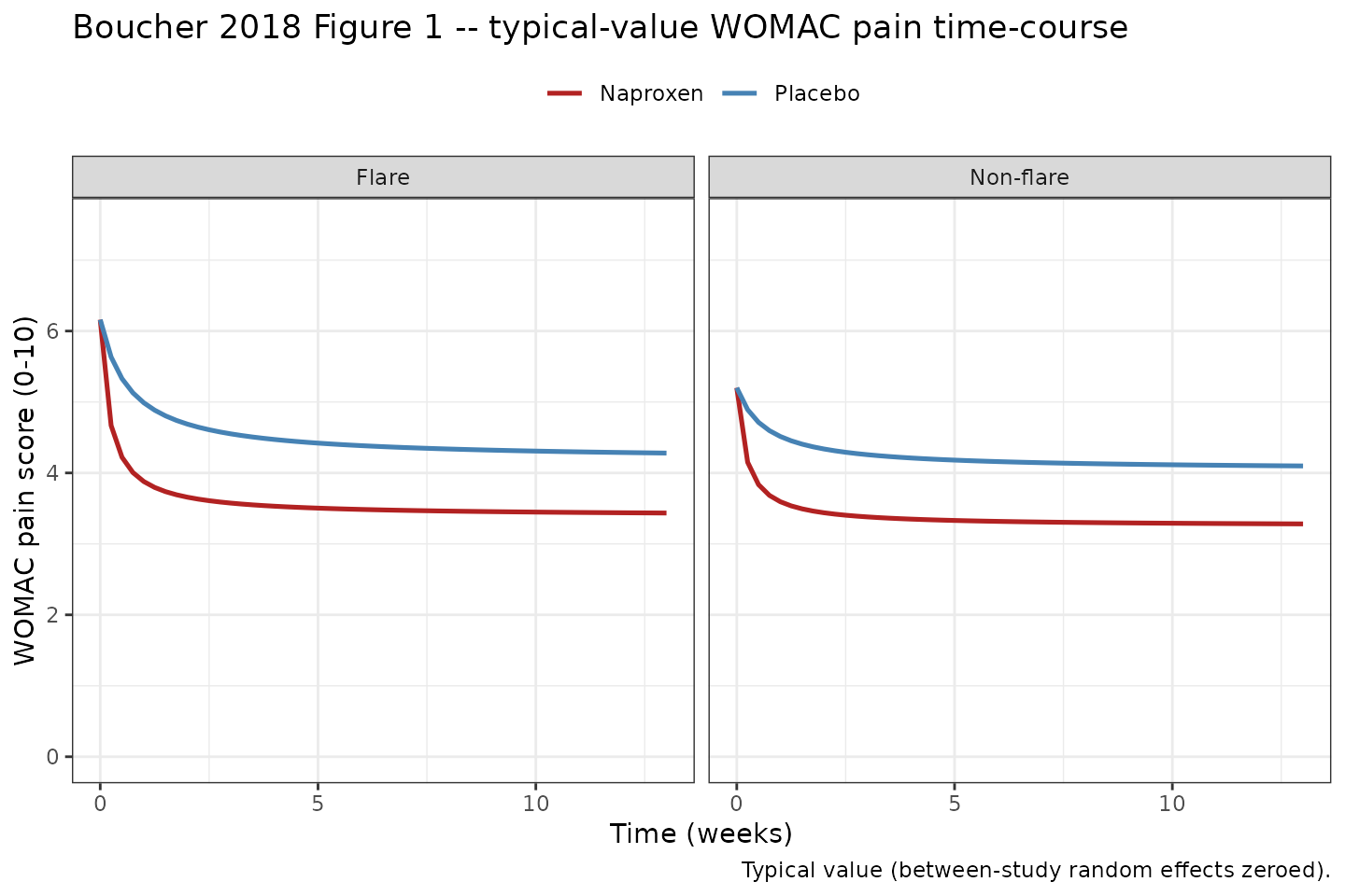
Replication of Boucher 2018 Figure 1: typical-value WOMAC pain time-course for naproxen and placebo, split by flare/non-flare design.
Replication: treatment difference over time (Boucher 2018 Figure 2)
Figure 2 of the paper plots the difference in mean WOMAC pain between treatments (naproxen minus placebo) over time, split by flare. Because baseline E0 does not depend on treatment, the difference is driven entirely by the Emax and ET50 treatment effects; naproxen’s shorter ET50 produces a faster, larger separation that then narrows slightly as both arms approach their maxima.
diff_df <- sim_fig1 |>
  dplyr::select(time, treatment, design, Cc) |>
  tidyr::pivot_wider(names_from = treatment, values_from = Cc) |>
  dplyr::mutate(diff = Naproxen - Placebo)

ggplot(diff_df, aes(x = time, y = diff, colour = design)) +
  geom_line(linewidth = 0.9) +
  geom_hline(yintercept = 0, linetype = "dotted") +
  scale_colour_manual(values = c("Flare" = "darkorange",
                                 "Non-flare" = "darkgreen")) +
  labs(
    x = "Time (weeks)",
    y = "WOMAC pain difference (naproxen - placebo)",
    colour = NULL,
    title = "Boucher 2018 Figure 2 -- treatment difference over time",
    caption = "Negative = greater pain reduction on naproxen than placebo."
  ) +
  theme_bw() +
  theme(legend.position = "top")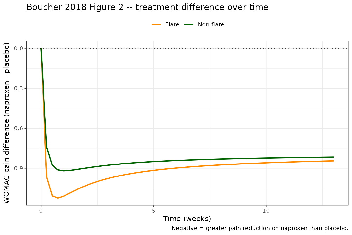
Replication of Boucher 2018 Figure 2: typical-value treatment difference (naproxen minus placebo) in WOMAC pain over time, split by flare design.
Comparison against published estimates (Boucher 2018 Table 3)
Table 3 reports the longitudinal-model treatment difference (naproxen minus placebo) at weeks 2, 6, and 12, alongside the landmark random-effects estimates. The table below compares the typical-value difference computed from the packaged model against the published NONMEM longitudinal point estimates and the landmark point estimates. The model reproduces the published longitudinal point estimates to the reported two decimals.
model_diff <- function(flare, wk) {
  evp <- as.data.frame(rxode2::et(wk)); evp$id <- 1L; evp$NAPROXEN <- 0L; evp$FLARE <- flare
  evn <- as.data.frame(rxode2::et(wk)); evn$id <- 1L; evn$NAPROXEN <- 1L; evn$FLARE <- flare
  cp <- rxode2::rxSolve(mod_typ, evp, returnType = "data.frame")$Cc
  cn <- rxode2::rxSolve(mod_typ, evn, returnType = "data.frame")$Cc
  cn - cp
}

tab3 <- tibble::tibble(
  Design = rep(c("Non-flare", "Flare"), each = 3),
  Week   = rep(c(2, 6, 12), times = 2),
  `Model (this package)` = round(c(
    model_diff(0L, 2), model_diff(0L, 6), model_diff(0L, 12),
    model_diff(1L, 2), model_diff(1L, 6), model_diff(1L, 12)
  ), 2),
  `Published NONMEM longitudinal` = c(-0.90, -0.84, -0.82, -1.03, -0.90, -0.85),
  `Published landmark`            = c(-1.08, -0.95, -0.62, -1.06, -0.99, -0.67)
)
#> ℹ omega/sigma items treated as zero: 'eta_study_e0', 'eta_study_emax'
#> ℹ omega/sigma items treated as zero: 'eta_study_e0', 'eta_study_emax'
#> ℹ omega/sigma items treated as zero: 'eta_study_e0', 'eta_study_emax'
#> ℹ omega/sigma items treated as zero: 'eta_study_e0', 'eta_study_emax'
#> ℹ omega/sigma items treated as zero: 'eta_study_e0', 'eta_study_emax'
#> ℹ omega/sigma items treated as zero: 'eta_study_e0', 'eta_study_emax'
#> ℹ omega/sigma items treated as zero: 'eta_study_e0', 'eta_study_emax'
#> ℹ omega/sigma items treated as zero: 'eta_study_e0', 'eta_study_emax'
#> ℹ omega/sigma items treated as zero: 'eta_study_e0', 'eta_study_emax'
#> ℹ omega/sigma items treated as zero: 'eta_study_e0', 'eta_study_emax'
#> ℹ omega/sigma items treated as zero: 'eta_study_e0', 'eta_study_emax'
#> ℹ omega/sigma items treated as zero: 'eta_study_e0', 'eta_study_emax'

knitr::kable(
  tab3, digits = 2,
  caption = "Treatment difference (naproxen - placebo) in WOMAC pain at weeks 2, 6, 12: packaged model vs Boucher 2018 Table 3 (NONMEM longitudinal and landmark point estimates)."
)| Design | Week | Model (this package) | Published NONMEM longitudinal | Published landmark |
|---|---|---|---|---|
| Non-flare | 2 | -0.90 | -0.90 | -1.08 |
| Non-flare | 6 | -0.84 | -0.84 | -0.95 |
| Non-flare | 12 | -0.82 | -0.82 | -0.62 |
| Flare | 2 | -1.03 | -1.03 | -1.06 |
| Flare | 6 | -0.90 | -0.90 | -0.99 |
| Flare | 12 | -0.85 | -0.85 | -0.67 |
# Regression guard: the model must match the published longitudinal estimates.
stopifnot(max(abs(tab3$`Model (this package)` -
                    tab3$`Published NONMEM longitudinal`)) <= 0.01)
The largest model-vs-published difference is within 0.01 WOMAC units of the NONMEM longitudinal estimate, confirming the structural model and parameter values were transcribed correctly. The landmark estimates differ more at week 12 (especially non-flare, where only two trials reported week-12 data); the paper notes that the week-12 landmark and longitudinal estimates are less comparable than the earlier timepoints because of the small number of contributing trials.
Between-study stochastic envelope
Because the between-study random effects eta1 (on E0, SD
0.62) and eta2 (on Emax, SD 0.74) are retained in the
model, the full model can simulate a distribution of study-arm-mean
trajectories. The envelope below draws 400 hypothetical naproxen
flare-design study arms and shows the median and 5th-95th percentile
band of arm-mean WOMAC pain over time. The simulation scope is
study-arm-mean WOMAC pain, not individual-patient
pain.
set.seed(20180420)
n_arm_sim <- 400L

ev_env <- as.data.frame(rxode2::et(tgrid))
ev_env <- ev_env[rep(seq_len(nrow(ev_env)), times = n_arm_sim), , drop = FALSE]
ev_env$id <- rep(seq_len(n_arm_sim), each = length(tgrid))
ev_env$NAPROXEN <- 1L
ev_env$FLARE    <- 1L

sim_env <- rxode2::rxSolve(mod_full, events = ev_env) |> as.data.frame()
#> ℹ parameter labels from comments will be replaced by 'label()'

env_summary <- sim_env |>
  dplyr::group_by(time) |>
  dplyr::summarise(
    median = median(Cc),
    lo     = quantile(Cc, 0.05),
    hi     = quantile(Cc, 0.95),
    .groups = "drop"
  )

ggplot(env_summary, aes(x = time)) +
  geom_ribbon(aes(ymin = lo, ymax = hi), alpha = 0.25, fill = "firebrick") +
  geom_line(aes(y = median), colour = "firebrick", linewidth = 0.9) +
  coord_cartesian(ylim = c(0, 9)) +
  labs(
    x = "Time (weeks)", y = "Study-arm-mean WOMAC pain (0-10)",
    title = "Between-study envelope -- naproxen flare-design arms",
    caption = "400 simulated study arms; between-study SD on E0 = 0.62, on Emax = 0.74."
  ) +
  theme_bw()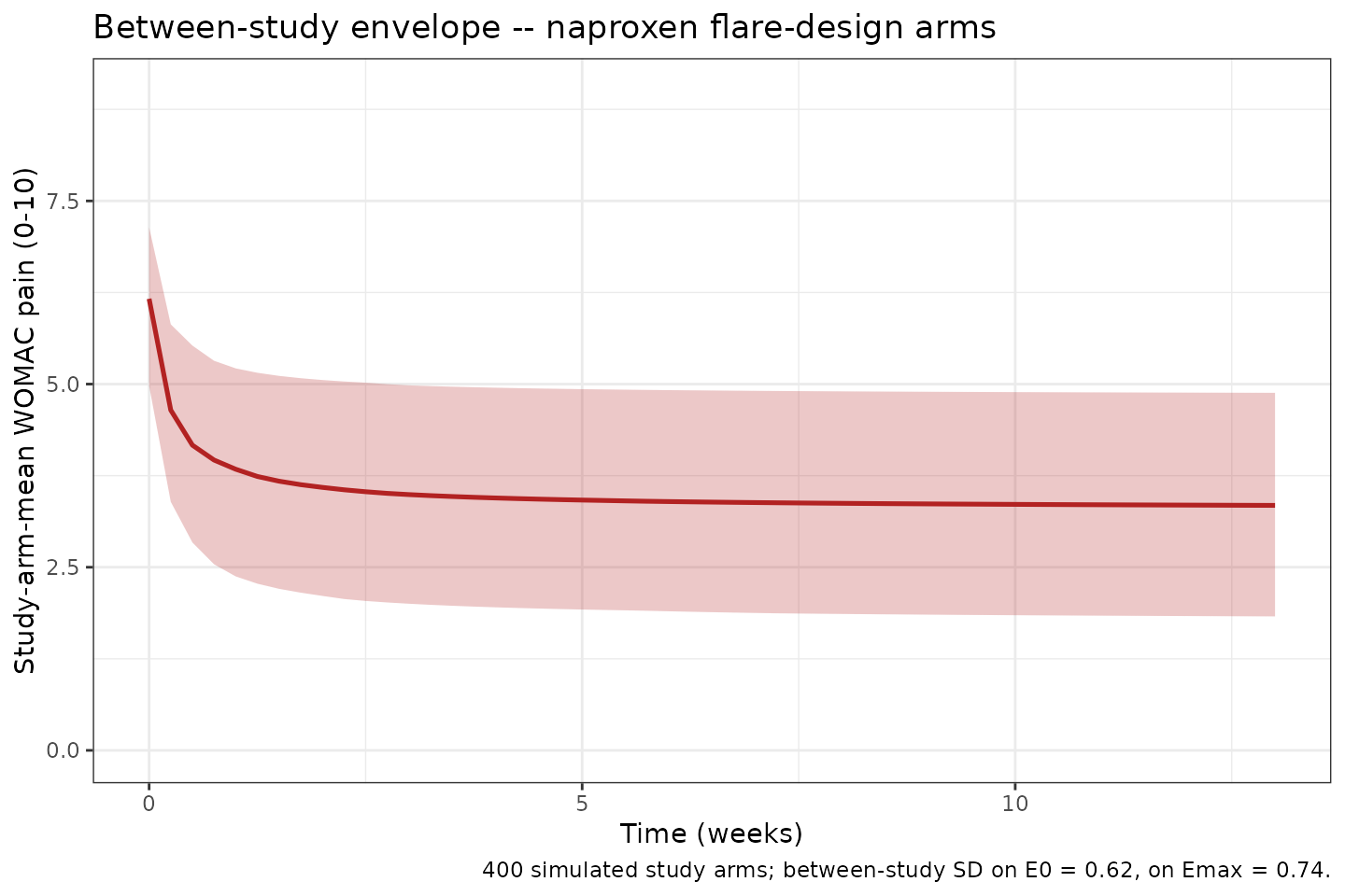
Between-study envelope: median and 5th-95th percentile of simulated naproxen flare-design study-arm-mean WOMAC pain over time (400 arms, between-study random effects active).
The between-study variability widens the band of plausible arm-mean
trajectories around the typical-value naproxen flare curve from Figure 1
(baseline ~6.2, approaching ~3.4). The residual error term
(addSd, sigma fixed to 1) is not added
here: in the source model the per-observation residual SD is the
observed standard error of each study-arm mean
(SD_ijk / sqrt(n_ijk)), so reproducing the published
residual weighting requires per-arm-per-timepoint SE values from the
(unavailable) dataset. The envelope above therefore reflects
between-study structural variability only.
Assumptions and deviations
MBMA, not population PK/PD. This is a model-based meta-analysis at the study-arm level. Each data point is the mean WOMAC pain in a trial arm at a timepoint, not an individual measurement. The model is intended for simulating study-arm-mean WOMAC pain time-courses and is not suitable for individual-subject simulation. The output
Ccis overloaded (per the nlmixr2lib single-output convention) to carry the WOMAC pain score and is not a drug concentration.Between-study random effects encoded as study-level etas. The paper’s
eta1(on E0) andeta2(on Emax) are between-study/arm random effects capturing the correlation between repeated timepoints within a study arm. They are encoded aseta_study_e0andeta_study_emaxto flag them as MBMA study-level variability rather than individual between-subject variability.checkModelConventions()warns that these etas have no matching structural fixed-effect parameter named_study_e0/_study_emax; this is expected for the MBMA between-study naming convention (SKILL Phase-1 Step-3a) and is not a defect. Theini()value is the variance (tau^2); Table 2 reportstau(the SD): s1 = 0.62, s2 = 0.74.Parameter source: the NONMEM column of Table 2. The paper fit the same Emax model in NONMEM, BUGS, and R(NLME) with closely agreeing estimates and produced its diagnostics from the NONMEM output. The NONMEM column was used throughout; the BUGS and R estimates differ only in the second decimal (and in s1, where BUGS reported 0.86 vs NONMEM/R 0.62).
Flare-by-treatment interaction excluded. Boucher 2018 Eq 5 added a flare-by-treatment covariate on the naproxen Emax; it was tested and found not significant, and Table 2 / Table 3 estimates exclude it. The model uses the additive Eq 3.
ET50 parameterized on the log scale. The paper fit
ln(ET50)to keep ET50 positive.let50 = -0.37is the placeboln(ET50p)(ET50 = 0.69 week);e_naproxen_et50 = -1.17is the additive naproxen shift on the log scale, giving naproxen ET50 = exp(-0.37 - 1.17) = 0.21 week. Both ET50 estimates are below one week, earlier than any post-dose observation in the studies (Boucher 2018 Results), so the onset portion of the curve is an extrapolation below the observed time grid.Residual error: sigma fixed to 1, per-arm SE weighting external. Eq 1 weights each study-arm-mean residual by its observed standard error (variance
SD_ijk^2 / n_ijk); because the weights were the observed SEs, the paper fixed sigma to 1. The model file exposesaddSd = fixed(1)and leaves the per-arm SE reweighting to downstream simulation code, mirroring theVargo_2014MBMA pattern. The stochastic-envelope figure therefore shows between-study structural variability only and does not add residual noise.Study-arm covariates documented inline.
FLARE(design indicator) andNAPROXEN(treatment indicator) are study-arm-level properties, not individual-level covariates. They are documented incovariateDatarather than added to the individual-level pop-PK register ininst/references/covariate-columns.md, following theVargo_2014_statins_ezetimibe_mbma/Sadouki_2025precedent for MBMA / multi-drug study-arm covariates.checkModelConventions()warns that these are not in the canonical register; this is expected.No parameter-uncertainty intervals reproduced. Table 3 reports 95% confidence/credible intervals on the treatment differences. The packaged model carries point estimates only (no parameter covariance matrix is published), so the comparison table reproduces the point estimates, not the intervals.
Total patient count unavailable. The per-trial sample sizes are in Supplementary Table S2, which was not on disk;
population$n_subjectsisNA. The number of trials (18) and the flare/non-flare split (12/6) are from the main-text “Example dataset” section.