Methotrexate (Joerger 2006)
Source:vignettes/articles/Joerger_2006_methotrexate.Rmd
Joerger_2006_methotrexate.RmdModel and source
#> ℹ parameter labels from comments will be replaced by 'label()'- Citation: Joerger M, Huitema ADR, van den Bongard HJGD, Baas P, Schornagel JH, Schellens JHM, Beijnen JH. Determinants of the elimination of methotrexate and 7-hydroxy-methotrexate following high-dose infusional therapy to cancer patients. Br J Clin Pharmacol. 2006;62(1):71-80. doi:10.1111/j.1365-2125.2005.02513.x
- Description: Population PK model for methotrexate (MTX) and its principal circulating metabolite 7-hydroxy-methotrexate (7-OH-MTX) in adult cancer patients receiving high-dose intravenous MTX therapy (Joerger 2006). Joint parent + metabolite model: linear 3-compartment MTX (central + two peripheral compartments) with first-order elimination from the central compartment, feeding a linear 2-compartment 7-OH-MTX disposition through a fixed metabolic fraction of 10 percent. Additive-linear covariate effects of baseline creatinine clearance (Cockcroft-Gault, raw mL/min, truncated at 140), concurrent benzimidazole-class proton-pump-inhibitor comedication, and prior NSAID administration on both MTX and 7-OH-MTX total clearance.
- Article: https://doi.org/10.1111/j.1365-2125.2005.02513.x
Population
The model was fit to 76 adult cancer patients (62 male / 14 female; age range 17.1-77.0 years, median 51.1 years; BSA 1.56-2.45 m^2, median 1.94 m^2) who received 304 cycles of high-dose intravenous methotrexate (HDMTX) at The Netherlands Cancer Institute. Indications included malignant pleural mesothelioma (n = 29), gastro-oesophageal cancer (n = 20), non-Hodgkin lymphoma (n = 12), head and neck cancer (n = 10), choriocarcinoma (n = 2), and one patient each with acute lymphocytic leukaemia, trophoblastic tumour, and osteosarcoma. Baseline raw Cockcroft-Gault creatinine clearance ranged 40-140 mL/min (median 87.5 mL/min, values above 140 truncated). MTX doses ranged 300 mg/m^2 to 12 g/m^2 over a 1-24 h infusion; 80 percent of cycles were 1000-5000 mg/m^2 over a 1-6 h infusion. Supportive therapy was uniform across the cohort (aggressive hydration, urine alkalinization, oral leucovorin rescue starting 24 h post-MTX). Concurrent benzimidazole-class proton-pump inhibitors (omeprazole 20-40 mg daily in 10 patients, lansoprazole 30 mg daily in 3) and prior NSAIDs (diclofenac in 5, ibuprofen in 1) were the retained covariates. See Joerger 2006 Table 1 (page 74) for baseline demographics.
The same metadata is available programmatically via
readModelDb("Joerger_2006_methotrexate")$population.
Source trace
The per-parameter origin is recorded as an in-file comment next to
each ini() entry in
inst/modeldb/specificDrugs/Joerger_2006_methotrexate.R. The
table below collects them in one place for review.
| Equation / parameter | Value | Source location |
|---|---|---|
lcl (baseline CL_MTX at median CRCL) |
8.85 L/h | Table 2 (p. 76) “Full data set Estimate”; Eq 1 baseline at CRCL = 87, PPI = 0, NSAID = 0 |
lvc (V_CENTRAL_MTX) |
23.0 L | Table 2 (p. 76) |
lvp (V_PERIPHERAL-1_MTX) |
185 L | Table 2 (p. 76) |
lvp2 (V_PERIPHERAL-2_MTX) |
5.34 L | Table 2 (p. 76) |
lq (Q1) |
0.444 L/h | Table 2 (p. 76) |
lq2 (Q2) |
0.716 L/h | Table 2 (p. 76) |
lcl_7ohmtx (baseline CL_7-OH-MTX at median CRCL) |
2 L/h | Table 2 (p. 76); Eq 2 baseline |
lvc_7ohmtx (V_CENTRAL_7-OH-MTX) |
21.6 L | Table 2 (p. 76) |
lvp_7ohmtx (V_PERIPHERAL_7-OH-MTX) |
27.7 L | Table 2 (p. 76) |
lq_7ohmtx (Q3) |
0.429 L/h | Table 2 (p. 76) |
lfm (metabolic fraction MTX -> 7-OH-MTX) |
0.10 (FIXED) | Results p. 75: assumed 10 percent per literature |
e_crcl_cl (slope on CRCL) |
0.0423 L/h per mL/min | Eq 1 (p. 77); sign corrected (see Errata) |
e_ppi_cl (PPI effect on CL_MTX) |
-2.45 L/h | Eq 1 (p. 77) |
e_nsaid_cl (NSAID effect on CL_MTX) |
-1.46 L/h | Eq 1 (p. 77) |
e_crcl_cl_7ohmtx (slope on CRCL) |
0.0123 L/h per mL/min | Eq 2 (p. 77); sign corrected (see Errata) |
e_ppi_cl_7ohmtx (PPI effect on CL_7-OH-MTX) |
-0.369 L/h | Eq 2 (p. 77) |
e_nsaid_cl_7ohmtx (NSAID effect on CL_7-OH-MTX) |
-0.357 L/h | Eq 2 (p. 77) |
| IIV CV percent (Table 2 p. 76) | CL_MTX 19.6, V_P-2_MTX 31.0, Q1 32.0, CL_7-OH-MTX 31.0, V_C_7-OH-MTX 8.22, V_P_7-OH-MTX 41.4, Q3 27.1 | Table 2; converted to log-normal variance via omega^2 = log(1 + CV^2) |
| Proportional residual MTX | 52.3 percent CV | Table 2 (p. 76); additive-on-log-scale = proportional in linear space |
| Proportional residual 7-OH-MTX | 57.1 percent CV | Table 2 (p. 76) |
d/dt(central) (3-cmt parent disposition) |
n/a | Figure 2 (p. 75): linear 3-compartment MTX |
d/dt(central_7ohmtx) (2-cmt metabolite, fed by fm * kel
* central) |
n/a | Figure 2 (p. 75); 10 percent metabolic flux per Results p. 75 |
Virtual cohort
Original observed data are not publicly available. The cohort simulated here uses the most common HDMTX regimen in the source paper – 3000 mg of methotrexate over a 3 h intravenous infusion – across four comedication arms (no comedication / PPI only / NSAID only / both), with baseline creatinine clearance drawn from a truncated normal centered at the cohort median 87 mL/min.
set.seed(20260627L)

make_cohort <- function(n, ppi, nsaid, id_offset = 0L) {
  # Truncated normal for raw Cockcroft-Gault CRCL: median 87, SD chosen to
  # span the source range (40-140 mL/min). Truncate at 140 per the paper.
  crcl_draw <- pmin(pmax(rnorm(n, mean = 87, sd = 25), 40), 140)

  ids <- id_offset + seq_len(n)

  # Methotrexate MW 454.4 g/mol; 3000 mg = 6.603 mmol = 6603 umol.
  # Modelled dose units are umol (matching plasma concentration units).
  mtx_dose_umol <- 3000 / 454.4 * 1000
  dose_rows <- tibble(
    id     = ids,
    time   = 0,
    evid   = 1L,
    amt    = mtx_dose_umol,            # umol
    rate   = mtx_dose_umol / 3,        # umol/h => 3 h infusion
    cmt    = "central",
    CRCL   = crcl_draw,
    CONMED_PPI   = ppi,
    CONMED_NSAID = nsaid
  )

  # Dense observation grid: fine through end of infusion / distribution,
  # then logarithmic spacing for the long terminal phase to support Figure 1
  # replication and 24 h / 48 h NCA windows.
  obs_times <- sort(unique(c(
    seq(0, 6, by = 0.5),
    seq(7, 12, by = 1),
    seq(15, 72, by = 3),
    seq(84, 168, by = 12)
  )))

  obs_rows <- tibble(
    id     = rep(ids, each = length(obs_times)),
    time   = rep(obs_times, times = n),
    evid   = 0L,
    amt    = NA_real_,
    rate   = NA_real_,
    cmt    = "Cc",
    CRCL   = rep(crcl_draw, each = length(obs_times)),
    CONMED_PPI   = ppi,
    CONMED_NSAID = nsaid
  )

  bind_rows(dose_rows, obs_rows) |>
    arrange(id, time, desc(evid))
}

n_per_arm <- 100L
events <- bind_rows(
  make_cohort(n_per_arm, ppi = 0, nsaid = 0, id_offset =   0L) |>
    mutate(treatment = "Neither PPI nor NSAID"),
  make_cohort(n_per_arm, ppi = 1, nsaid = 0, id_offset = 100L) |>
    mutate(treatment = "PPI only"),
  make_cohort(n_per_arm, ppi = 0, nsaid = 1, id_offset = 200L) |>
    mutate(treatment = "Prior NSAID only"),
  make_cohort(n_per_arm, ppi = 1, nsaid = 1, id_offset = 300L) |>
    mutate(treatment = "PPI + prior NSAID")
)

stopifnot(!anyDuplicated(unique(events[, c("id", "time", "evid")])))
Simulation
mod <- readModelDb("Joerger_2006_methotrexate")

sim <- rxode2::rxSolve(
  mod,
  events = events,
  keep   = c("treatment")
) |>
  as.data.frame() |>
  as_tibble()
#> ℹ parameter labels from comments will be replaced by 'label()'
Replicate Figure 1: mean MTX concentration-time profile
Figure 1 of Joerger 2006 (page 75) plots
ln(MTX concentration) vs. time for the cohort mean and two
outliers, both of whom received 3 g of MTX as a 3 h infusion. The mean
profile descends slowly out to roughly 500 h, reflecting the deep MTX
peripheral compartment (V_PERIPHERAL-1_MTX = 185 L) which re-supplies
the central compartment via Q1 = 0.444 L/h after the rapid elimination
clears the bolus. The simulation below replicates that mean profile for
the no-comedication arm.
sim_mean <- sim |>
  filter(treatment == "Neither PPI nor NSAID", time > 0, !is.na(Cc)) |>
  group_by(time) |>
  summarise(
    mean_lnCc = mean(log(Cc), na.rm = TRUE),
    .groups   = "drop"
  )

ggplot(sim_mean, aes(time, mean_lnCc)) +
  geom_line() +
  labs(
    x       = "Time after start of MTX infusion (h)",
    y       = "Mean ln(MTX) (umol/L)",
    title   = "Replicates Figure 1 of Joerger 2006 (mean profile only).",
    caption = "Source: Joerger 2006 Figure 1 (page 75); 3 g MTX, 3 h IV infusion."
  ) +
  theme_bw()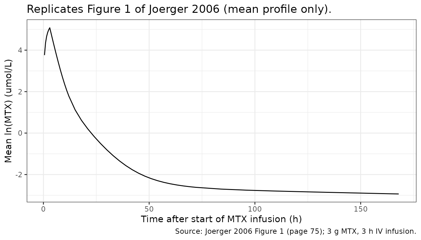
PKNCA validation
sim_nca <- sim |>
  filter(!is.na(Cc)) |>
  select(id, time, Cc, Cc_7ohmtx, treatment)

# Guarantee a time = 0 row per (id, treatment); MTX is administered IV so the
# pre-dose concentration is 0 for both analytes.
zero_rows <- sim_nca |>
  distinct(id, treatment) |>
  mutate(time = 0, Cc = 0, Cc_7ohmtx = 0)

sim_nca <- bind_rows(sim_nca, zero_rows) |>
  distinct(id, treatment, time, .keep_all = TRUE) |>
  arrange(id, treatment, time)

# MTX NCA
conc_mtx <- PKNCA::PKNCAconc(sim_nca, Cc ~ time | treatment + id)
# 7-OH-MTX NCA
conc_met <- PKNCA::PKNCAconc(sim_nca, Cc_7ohmtx ~ time | treatment + id)

dose_df <- events |>
  filter(evid == 1L) |>
  select(id, time, amt, treatment)

dose_obj <- PKNCA::PKNCAdose(dose_df, amt ~ time | treatment + id)

intervals <- data.frame(
  start       = 0,
  end         = Inf,
  cmax        = TRUE,
  tmax        = TRUE,
  aucinf.obs  = TRUE,
  half.life   = TRUE
)

nca_mtx <- PKNCA::pk.nca(PKNCA::PKNCAdata(conc_mtx, dose_obj, intervals = intervals))
nca_met <- PKNCA::pk.nca(PKNCA::PKNCAdata(conc_met, dose_obj, intervals = intervals))
nca_summary <- function(nca_res, analyte_label) {
  as.data.frame(nca_res$result) |>
    select(treatment, PPTESTCD, PPORRES) |>
    group_by(treatment, PPTESTCD) |>
    summarise(value = mean(PPORRES, na.rm = TRUE), .groups = "drop") |>
    pivot_wider(names_from = PPTESTCD, values_from = value) |>
    mutate(analyte = analyte_label) |>
    select(analyte, everything())
}

knitr::kable(
  bind_rows(
    nca_summary(nca_mtx, "MTX"),
    nca_summary(nca_met, "7-OH-MTX")
  ),
  caption = "Simulated NCA summary (cohort means) by comedication arm.",
  digits  = 3
)| analyte | treatment | adj.r.squared | aucinf.obs | clast.obs | clast.pred | cmax | half.life | lambda.z | lambda.z.n.points | lambda.z.time.first | lambda.z.time.last | r.squared | span.ratio | tlast | tmax |
|---|---|---|---|---|---|---|---|---|---|---|---|---|---|---|---|
| MTX | Neither PPI nor NSAID | 1.000 | 769.201 | 0.067 | 0.067 | 161.447 | 327.992 | 0.002 | 6.64 | 103.74 | 168 | 1 | 0.221 | 168 | 3.000 |
| MTX | PPI + prior NSAID | 0.999 | 1430.129 | 0.245 | 0.245 | 198.586 | 315.653 | 0.002 | 5.37 | 116.10 | 168 | 1 | 0.179 | 168 | 3.000 |
| MTX | PPI only | 1.000 | 1042.173 | 0.135 | 0.135 | 180.447 | 311.398 | 0.002 | 5.94 | 110.25 | 168 | 1 | 0.209 | 168 | 3.000 |
| MTX | Prior NSAID only | 1.000 | 929.279 | 0.103 | 0.103 | 173.545 | 323.754 | 0.002 | 6.09 | 107.91 | 168 | 1 | 0.207 | 168 | 3.000 |
| 7-OH-MTX | Neither PPI nor NSAID | 1.000 | 333.929 | 0.156 | 0.156 | 16.477 | 73.635 | 0.011 | 4.81 | 122.91 | 168 | 1 | 0.689 | 168 | 6.095 |
| 7-OH-MTX | PPI + prior NSAID | 1.000 | 564.845 | 0.509 | 0.509 | 15.114 | 83.244 | 0.009 | 3.82 | 134.16 | 168 | 1 | 0.462 | 168 | 8.960 |
| 7-OH-MTX | PPI only | 1.000 | 411.834 | 0.274 | 0.273 | 15.563 | 79.979 | 0.010 | 4.14 | 130.32 | 168 | 1 | 0.521 | 168 | 7.240 |
| 7-OH-MTX | Prior NSAID only | 1.000 | 425.233 | 0.264 | 0.263 | 16.555 | 78.589 | 0.010 | 4.52 | 125.76 | 168 | 1 | 0.614 | 168 | 6.870 |
Comparison against published 24-h and 48-h plasma concentrations
Table 3 of Joerger 2006 (page 76) reports geometric mean plasma concentrations of MTX and 7-OH-MTX at 24 h and 48 h in subgroups defined by concurrent benzimidazole or prior-NSAID exposure. The cohort received heterogeneous doses (300-12000 mg/m^2) and infusion durations (1-24 h), so the ratio between subgroups (+/- comedication) is the most directly comparable quantity; absolute concentrations are only approximately comparable because the simulation uses a single 3 g / 3 h dose. The table below pairs the simulated geometric-mean concentrations from the comedication arms with the published values from Table 3.
gmean <- function(x) exp(mean(log(x[x > 0]), na.rm = TRUE))

sim_24_48 <- sim |>
  filter(time %in% c(24, 48)) |>
  group_by(treatment, time) |>
  summarise(
    sim_mtx      = gmean(Cc),
    sim_7ohmtx   = gmean(Cc_7ohmtx),
    .groups      = "drop"
  )

published <- tibble::tribble(
  ~treatment,              ~time,  ~pub_mtx, ~pub_7ohmtx,
  "Neither PPI nor NSAID",   24L,    0.66,        2.52,    # "No benzimidazoles" row of Table 3
  "Neither PPI nor NSAID",   48L,    0.12,        0.72,
  "PPI only",                24L,    2.01,        4.47,    # "+ Benzimidazoles" row
  "PPI only",                48L,    0.25,        1.11,
  "Prior NSAID only",        24L,    0.98,        1.74,    # "Prior NSAIDs" row
  "Prior NSAID only",        48L,    0.17,        1.61,
  "PPI + prior NSAID",       24L,    NA_real_,    NA_real_,
  "PPI + prior NSAID",       48L,    NA_real_,    NA_real_
)

compare_tab <- sim_24_48 |>
  mutate(time = as.integer(time)) |>
  left_join(published, by = c("treatment", "time")) |>
  arrange(treatment, time)

knitr::kable(
  compare_tab,
  caption = "Simulated vs. Joerger 2006 Table 3 geometric mean plasma concentrations (umol/L). 'PPI + NSAID' has no published value (no Table 3 subgroup with both).",
  digits  = 3,
  col.names = c("Treatment", "Time (h)", "Simulated MTX", "Simulated 7-OH-MTX",
                "Published MTX (Table 3)", "Published 7-OH-MTX (Table 3)")
)| Treatment | Time (h) | Simulated MTX | Simulated 7-OH-MTX | Published MTX (Table 3) | Published 7-OH-MTX (Table 3) |
|---|---|---|---|---|---|
| Neither PPI nor NSAID | 24 | 0.846 | 3.540 | 0.66 | 2.52 |
| Neither PPI nor NSAID | 48 | 0.125 | 0.760 | 0.12 | 0.72 |
| PPI + prior NSAID | 24 | 4.186 | 7.446 | NA | NA |
| PPI + prior NSAID | 48 | 0.562 | 2.309 | NA | NA |
| PPI only | 24 | 1.883 | 4.792 | 2.01 | 4.47 |
| PPI only | 48 | 0.273 | 1.146 | 0.25 | 1.11 |
| Prior NSAID only | 24 | 1.414 | 5.061 | 0.98 | 1.74 |
| Prior NSAID only | 48 | 0.199 | 1.248 | 0.17 | 1.61 |
ratio_tab <- compare_tab |>
  filter(treatment %in% c("PPI only", "Prior NSAID only")) |>
  left_join(
    compare_tab |>
      filter(treatment == "Neither PPI nor NSAID") |>
      select(time, ref_sim_mtx = sim_mtx, ref_sim_7ohmtx = sim_7ohmtx,
             ref_pub_mtx = pub_mtx, ref_pub_7ohmtx = pub_7ohmtx),
    by = "time"
  ) |>
  mutate(
    sim_ratio_mtx     = sim_mtx    / ref_sim_mtx,
    pub_ratio_mtx     = pub_mtx    / ref_pub_mtx,
    sim_ratio_7ohmtx  = sim_7ohmtx / ref_sim_7ohmtx,
    pub_ratio_7ohmtx  = pub_7ohmtx / ref_pub_7ohmtx
  ) |>
  select(treatment, time, sim_ratio_mtx, pub_ratio_mtx,
         sim_ratio_7ohmtx, pub_ratio_7ohmtx)

knitr::kable(
  ratio_tab,
  caption = "Simulated vs. published ratios relative to the no-comedication subgroup (Joerger 2006 Table 3 'Ratio' row).",
  digits  = 2,
  col.names = c("Treatment", "Time (h)",
                "Sim ratio MTX", "Pub ratio MTX",
                "Sim ratio 7-OH-MTX", "Pub ratio 7-OH-MTX")
)| Treatment | Time (h) | Sim ratio MTX | Pub ratio MTX | Sim ratio 7-OH-MTX | Pub ratio 7-OH-MTX |
|---|---|---|---|---|---|
| PPI only | 24 | 2.23 | 3.05 | 1.35 | 1.77 |
| PPI only | 48 | 2.18 | 2.08 | 1.51 | 1.54 |
| Prior NSAID only | 24 | 1.67 | 1.48 | 1.43 | 0.69 |
| Prior NSAID only | 48 | 1.59 | 1.42 | 1.64 | 2.24 |
Assumptions and deviations
Sign correction on the CRCL covariate effect (Equations 1 and 2). The printed equations on page 77 of Joerger 2006 are
CL_MTX = 8.85 + 0.0423 * (87 - CL_CREA) - 2.45 * PPI - 1.46 * NSAIDandCL_7-OH-MTX = 2 + 0.0123 * (87 - CL_CREA) - 0.369 * PPI - 0.357 * NSAID. Taken literally those equations make clearance decrease with rising creatinine clearance, which contradicts both the abstract (“Baseline creatinine clearance correlated with CL_MTX and CL_7-OH-MTX”) and the Discussion (“CL_CREA correlated with model-predicted CL_MTX and CL_7-OH-MTX, internally validating the presented population model”). The same Methods section (page 73) shows the linear-centering convention as(WT - 70)for body weight, i.e.(covariate - median), not(median - covariate). The model implements the operationally consistent forme_crcl_cl * (CRCL - 87)withe_crcl_cl = +0.0423and analogous for the metabolite, so higher CRCL produces higher clearance.Interoccasion variability on CL_MTX is not implemented. Joerger 2006 Table 2 reports IOV of 13.3 percent CV on CL_MTX (additive to the 19.6 percent CV IIV). nlmixr2’s native IOV requires an occasion column in the event table and a separate eta block tagged by occasion; the simulation cohort here uses single-occasion subjects, so IOV would not contribute. Stochastic simulations of cycle-to-cycle MTX exposure variability will under-estimate the spread by the IOV component; deterministic typical-value predictions are unaffected.
Residual error reported on log-scale, encoded as proportional. Joerger 2006 Methods (page 73) writes the residual model as
log(C_ij) = log(C_ij_pred) + eps_ij, which is additive-on-log-scale. In the linear-space convention used by nlmixr2lib’sprop()family the equivalent isy = ypred * (1 + eps); for sigma values at the 50 percent level the small-eps approximation is a few percent loose, but the published CVs are reproduced.Metabolic fraction fixed at 10 percent, not estimated. Joerger 2006 Results page 75 states “we assumed that 10 percent of MTX was metabolized to 7-OH-MTX, in accordance with literature data. Fixing the metabolic fraction to higher (up to 50 percent) or lower (down to 2 percent) values resulted in a decreased fit with an increased OFV.” The model wraps
lfminfixed()to preserve this provenance.Mole-equivalent stoichiometry. Plasma MTX and 7-OH-MTX are both reported in umol/L throughout the paper. The metabolic flux
fm * kel * centralis in MTX mass-equivalent units; treating the metabolite compartment as a 1:1 mole carry-over assumes negligible molecular-weight difference (MTX 454.4 g/mol, 7-OH-MTX 470.4 g/mol; +3.5 percent change). This is the same convention used by the source paper, which does not apply an explicit MW correction.Linear-additive covariate model on clearance. The paper uses linear centred covariates added to the baseline CL on the natural scale (not the log scale typical of nlmixr2 popPK conventions). The model preserves this by computing
tvcl = exp(lcl) + e_crcl_cl * (CRCL - 87) + ...and applying IIV multiplicatively around the linear-covariate-adjusted typical value:cl = tvcl * exp(etalcl). Within the source cohort’s covariate ranges (CRCL 40-140, PPI in {0,1}, NSAID in {0,1})tvclstays well above zero (minimum approximately 0.7 L/h for the metabolite and 3 L/h for the parent); extrapolating beyond these ranges – e.g. simulating a virtual patient with CRCL = 20 and both PPI = 1 and NSAID = 1 – can drivetvcltoward zero or negative and should be avoided.Subgroup absolute-concentration comparison is dose-confounded. Joerger 2006 Table 3 pools heterogeneous doses (300-12000 mg/m^2) and infusion durations (1-24 h) within each comedication subgroup. The simulation uses a single 3000 mg / 3 h IV dose, so absolute 24-h and 48-h concentrations are only approximately comparable to Table 3. The ratio between subgroups (
+/- PPIand+/- NSAID) is the more directly comparable quantity and is reported separately.No-Table-3 row for
PPI + prior NSAID. Joerger 2006 Table 3 does not report a subgroup with both PPI and NSAID, so the published-value column is blank for that arm.