Unfractionated heparin (Jia 2015)
Source:vignettes/articles/Jia_2015_unfractionatedHeparin.Rmd
Jia_2015_unfractionatedHeparin.RmdModel and source
- Citation: Jia Z, Tian G, Ren Y, Sun Z, Lu W, Hou X. Pharmacokinetic model of unfractionated heparin during and after cardiopulmonary bypass in cardiac surgery. J Transl Med. 2015 Feb 1;13:45. doi:10.1186/s12967-015-0404-5.
- Description: Two-compartment population PK model with first-order elimination for unfractionated heparin (UFH) administered as multiple intravenous bolus injections during cardiopulmonary bypass (CPB) in adult Chinese cardiac surgery patients (Jia 2015). Plasma UFH exposure was inferred from anti-FIIa chromogenic activity. No covariates were retained in the final model (age, body weight, and sex were tested via forward inclusion / backward elimination and none met the p < 0.001 retention threshold). Concentrations are reported in IU/mL of anti-FIIa activity; doses are in IU (1 mg UFH = 125 IU). The published model also describes instantaneous neutralization of central-compartment UFH at protamine sulfate dosing (see vignette for the simulation pattern); the structural ODEs here are the standard two-compartment IV bolus form.
- Article: https://doi.org/10.1186/s12967-015-0404-5 (open access in Journal of Translational Medicine 2015;13:45)
Population
The model was developed from 41 enrolled patients (32 completers) undergoing cardiopulmonary bypass (CPB) during cardiac surgery at Beijing Anzhen Hospital (Capital Medical University). Baseline characteristics from Table 1: body weight 66 kg (range 41-82), age 53.4 years (range 18-74), 19 females and 13 males (sex_female_pct = 59.4 percent), CPB time 2.04 h (range 0.95-3.29). Subjects with dysfunction of the kidney, liver, or blood coagulation were excluded prior to enrolment. UFH doses (Table 1): mean priming-fluid dose 8,516 IU (range 6,250-10,000); mean first bolus 24,805 IU (range 18,750-31,250); mean total dose 34,023 IU (range 25,000-45,000). Plasma anti-FIIa activity (used as the surrogate for plasma UFH concentration) was measured with the Heparin Chromogenic Activity Kit 820 on the ACL-TOP automated coagulation platform; pre-neutralization samples were diluted 1:29 in normal pooled platelet-poor plasma to bring activity into the assay range (0.0-0.6 IU/mL).
The same information is available programmatically via the model’s
population metadata
(readModelDb("Jia_2015_unfractionatedHeparin")$population).
Source trace
The per-parameter origin is recorded as an in-file comment next to
each ini() entry in
inst/modeldb/specificDrugs/Jia_2015_unfractionatedHeparin.R.
The table below collects them in one place for review.
| Equation / parameter | Value | Source location |
|---|---|---|
lcl (CL) |
log(1.18) – CL = 1.18 L/h | Table 2 row “CL_UFH, 1-order (L*h^-1)” |
lvc (V_UFH-C) |
log(3.04) – Vc = 3.04 L | Table 2 row “V_UFH-C (L)” |
lq (Q_UFH) |
log(0.171) – Q = 0.171 L/h | Table 2 row “Q_UFH (L*h^-1)” |
lvp (V_UFH-P) |
log(8.01) – Vp = 8.01 L | Table 2 row “V_UFH-P (L)” |
etalcl variance |
0.122 | Table 2 row “omega^2_CL(UFH, 1-order)” |
etalvc variance |
0.105 | Table 2 row “omega^2_V(UFH-C)” |
etalq variance |
0.0978 | Table 2 row “omega^2_Q(UFH)” |
| omega^2(V_UFH-P) | 0 (FIX) | Table 2 row “omega^2_V(UFH-P)” – no eta on lvp |
propSd |
sqrt(0.139) = 0.3728 | Table 2 row “sigma^2_pro(UFH)” (SD = sqrt(variance)) |
| sigma^2_add | 0 (FIX) | Table 2 row “sigma^2_add(UFH)” – additive component omitted |
d/dt(central) |
-kel*central - k12*central + k21*peripheral1 |
Eq. 1 (Methods, two-compartment ODE) |
d/dt(peripheral1) |
k12*central - k21*peripheral1 |
Eq. 2 (Methods, two-compartment ODE) |
| Concentration conversion | Cc = central / vc / 1000 |
Methods (dose in IU, vc in L, anti-FIIa activity reported in IU/mL) |
| IIV form | exponential P_i = P_pop * exp(eta_i)
|
Eq. 15 |
| Residual error form | hybrid Cobs = Cpred*(1+eps1) + eps2 with eps2=0
(FIX) |
Eq. 16 plus Table 2 footnote (sigma^2_add fixed at 0) |
Virtual cohort
Original individual data are not publicly available. The cohort below uses covariate distributions matching the Table 1 summaries: 32 completers with body weight uniform across the reported 41-82 kg range, sex 19 F / 13 M, age uniform across 18-74 years. UFH dosing follows the per-protocol regimen described in Methods: a body-weight-scaled initial bolus at 375 IU/kg (t = 0 h), a priming-fluid bolus of approximately 1 mg/kg = 125 IU/kg (t = 0.17 h), and protamine sulfate neutralization at the end of CPB (median CPB time 2.04 h).
set.seed(20150201)  # paper online publication date

n_subj <- 32L

cohort <- tibble(
  id        = seq_len(n_subj),
  WT        = round(runif(n_subj, 41, 82), 1),
  age_years = round(runif(n_subj, 18, 74), 1),
  SEXF      = c(rep(1L, 19), rep(0L, 13)),
  cpb_h     = round(runif(n_subj, 0.95, 3.29), 2)
) |>
  mutate(
    dose_initial_iu = round(WT * 375),     # initial bolus 375 IU/kg
    dose_priming_iu = round(WT * 125)      # priming fluid bolus 1 mg/kg = 125 IU/kg
  )

knitr::kable(
  head(cohort, 6) |> mutate(across(where(is.numeric), ~ signif(.x, 4))),
  caption = "First six simulated subjects (body weight, sex, CPB duration, per-subject UFH bolus sizes)."
)| id | WT | age_years | SEXF | cpb_h | dose_initial_iu | dose_priming_iu |
|---|---|---|---|---|---|---|
| 1 | 72.7 | 24.6 | 1 | 1.89 | 27260 | 9088 |
| 2 | 49.9 | 66.2 | 1 | 1.06 | 18710 | 6238 |
| 3 | 69.2 | 52.3 | 1 | 1.27 | 25950 | 8650 |
| 4 | 81.8 | 27.4 | 1 | 1.63 | 30680 | 10220 |
| 5 | 56.3 | 28.0 | 1 | 1.77 | 21110 | 7038 |
| 6 | 56.6 | 63.7 | 1 | 3.23 | 21220 | 7075 |
Simulation
The packaged model is the two-compartment IV bolus structural model
(Eq. 1-2 of Methods). The protamine neutralization manoeuvre at the end
of CPB is modelled by post-processing: at t = Tneu the
central compartment is reset to zero (excess protamine instantly
inactivates circulating anti-FIIa activity) while the peripheral
compartment is left unchanged, after which the model is restarted with
the saved peripheral amount as the initial condition. This matches the
Methods description (“at the time of neutralization, the value of XUFH-C
was instantly set to 0, whereas the value of XUFH-P at that moment was
documented automatically as the new initial condition”).
For the validation here, the focus is on the during-CPB phase (which
the structural model handles directly) plus a single-subject
demonstration of the post-CPB heparin-rebound phase that combines two
sequential rxSolve calls.
mod <- readModelDb("Jia_2015_unfractionatedHeparin")

# Build per-subject during-CPB events: initial bolus at t = 0, priming-fluid
# bolus at t = 0.17 h (10 minutes after the first sample per the Methods
# protocol), then a dense observation grid from t = 0 to t = 2.04 h
# (median CPB duration).
dose_initial <- cohort |>
  transmute(id, time = 0,    amt = dose_initial_iu, evid = 1L, cmt = "central", WT, SEXF)
dose_priming <- cohort |>
  transmute(id, time = 0.17, amt = dose_priming_iu, evid = 1L, cmt = "central", WT, SEXF)

obs_times <- seq(0, 2.04, by = 0.02)
obs_rows <- cohort |>
  tidyr::expand_grid(time = obs_times) |>
  transmute(id, time, amt = 0, evid = 0L, cmt = "central", WT, SEXF)

events_cpb <- dplyr::bind_rows(dose_initial, dose_priming, obs_rows) |>
  dplyr::arrange(id, time, dplyr::desc(evid))

# Typical-value simulation (no eta) for figure overlays; stochastic
# simulation for the VPC-style spread.
sim_typ <- rxode2::rxSolve(
  mod |> rxode2::zeroRe(),
  events = events_cpb,
  keep = c("WT", "SEXF"),
  addDosing = FALSE
) |> as.data.frame()
#> ℹ parameter labels from comments will be replaced by 'label()'
#> ℹ omega/sigma items treated as zero: 'etalcl', 'etalvc', 'etalq'
#> Warning: multi-subject simulation without without 'omega'

sim_vpc <- rxode2::rxSolve(
  mod,
  events = events_cpb,
  keep = c("WT", "SEXF"),
  addDosing = FALSE,
  nSub = 1L
) |> as.data.frame()
#> ℹ parameter labels from comments will be replaced by 'label()'
Initial half-life check (Discussion: “approximate initial half-life of 90 min”)
The Discussion reports an approximate initial half-life of 90 min. Two- compartment math from the typical population estimates predicts an alpha (distribution) half-life of about 93 min, which matches the paper. This is the strongest single check on the structural parameter set.
cl <- 1.18; vc <- 3.04; q <- 0.171; vp <- 8.01
kel <- cl / vc
k12 <- q  / vc
k21 <- q  / vp
kbar <- kel + k12 + k21
disc <- sqrt(kbar^2 - 4 * kel * k21)
alpha <- (kbar + disc) / 2
beta  <- (kbar - disc) / 2

knitr::kable(
  tibble(
    quantity = c("alpha (1/h)", "beta (1/h)",
                 "alpha half-life (min)", "beta half-life (h)"),
    value    = c(signif(alpha, 4), signif(beta, 4),
                 signif(log(2) / alpha * 60, 4),
                 signif(log(2) / beta, 4))
  ),
  caption = "Analytic two-compartment eigenvalues from the published typical population estimates. The alpha half-life of approximately 93 min agrees with the Discussion claim of an initial half-life around 90 min."
)| quantity | value |
|---|---|
| alpha (1/h) | 0.44720 |
| beta (1/h) | 0.01853 |
| alpha half-life (min) | 92.99000 |
| beta half-life (h) | 37.41000 |
Replicate Figure 2A (anti-FIIa activity during CPB)
Figure 2A of Jia 2015 shows plasma anti-FIIa activity during CPB. The Discussion summarises the typical plateau as 2-19 IU/mL with a median end-of- CPB activity of 4.8 IU/mL. The simulated typical-value profile below overlays the cohort and confirms a comparable plateau range.
ggplot(sim_typ, aes(time, Cc, group = id)) +
  geom_line(alpha = 0.4, colour = "steelblue") +
  scale_y_log10() +
  labs(
    x       = "Time after first UFH bolus (h)",
    y       = "Plasma anti-FIIa activity (IU/mL)",
    title   = "Simulated during-CPB anti-FIIa activity",
    caption = "Reproduces the typical-value behaviour of Figure 2A of Jia 2015."
  ) +
  theme_minimal()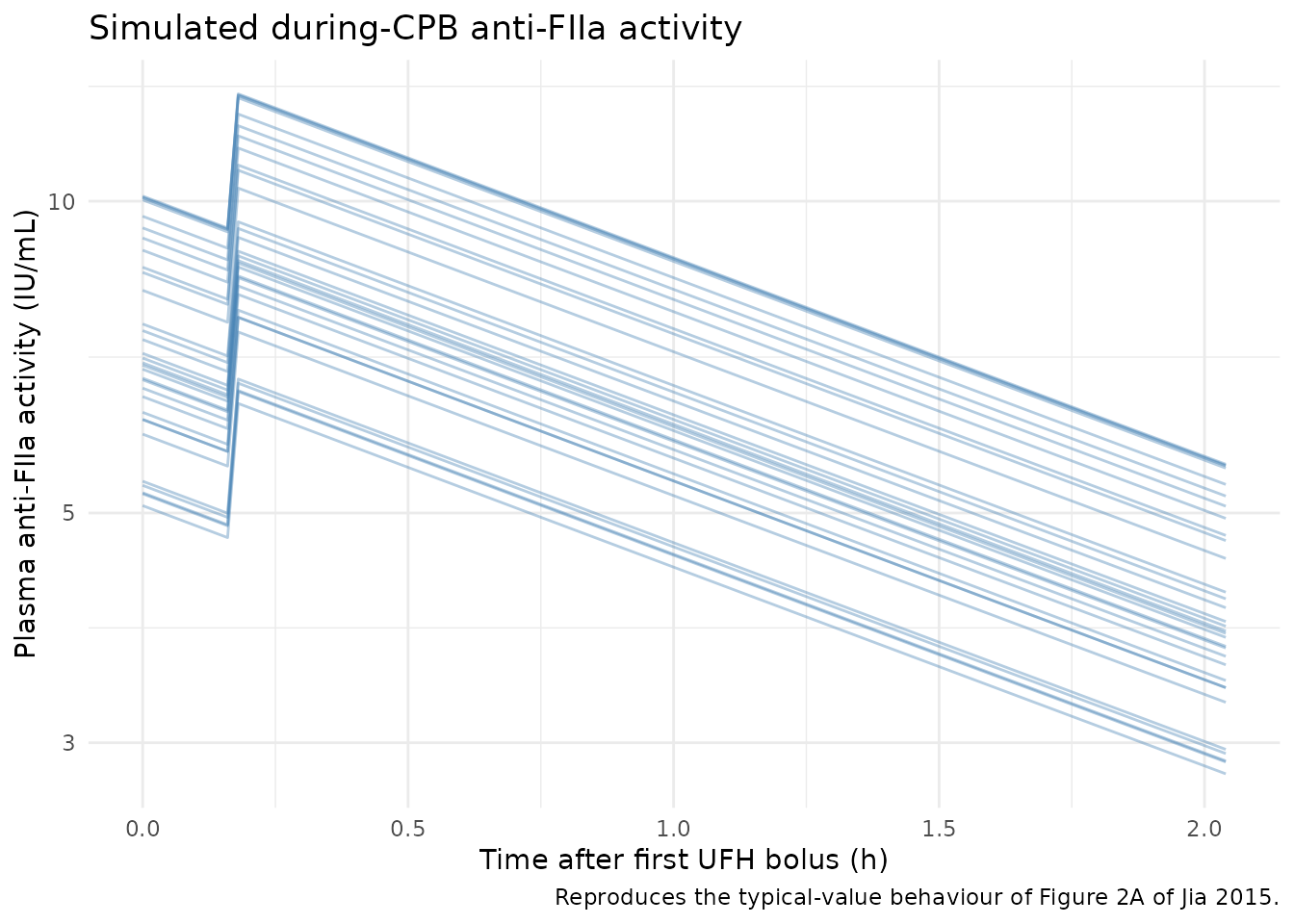
Replicates Figure 2A of Jia 2015: simulated plasma anti-FIIa activity during CPB. Each thin line is one virtual subject (typical-value parameters, body-weight-scaled bolus). The two boluses (t = 0 and t = 0.17 h) produce a rising-then-decaying anti-FIIa profile; the median end-of-CPB activity sits in the published 2-19 IU/mL plateau range.
end_of_cpb <- sim_typ |>
  group_by(id) |>
  filter(time == max(time)) |>
  ungroup() |>
  summarise(
    n        = n(),
    Cc_min   = min(Cc),
    Cc_med   = median(Cc),
    Cc_max   = max(Cc)
  )

knitr::kable(
  end_of_cpb |> mutate(across(where(is.numeric), ~ signif(.x, 4))),
  caption = "Simulated end-of-CPB anti-FIIa activity across the virtual cohort. Discussion of Jia 2015 reports a typical plateau of 2-19 IU/mL with a median end-of-CPB activity of 4.8 IU/mL."
)| n | Cc_min | Cc_med | Cc_max |
|---|---|---|---|
| 32 | 2.8 | 3.867 | 5.572 |
Heparin rebound after protamine neutralization (single-subject demo)
Protamine sulfate neutralizes circulating UFH instantaneously. The Methods encode this as setting the central-compartment amount to zero at the neutralization time while leaving the peripheral compartment unchanged. After neutralization, UFH that had distributed into the peripheral compartment slowly redistributes back into the central compartment, producing a measurable post-CPB heparin-rebound peak (Figure 2B of Jia 2015, characterised in Discussion as a peak of 0.04 IU/mL around 8 h after neutralization).
The demo below stitches two sequential rxSolve calls for
a typical 66 kg subject:
- Simulate during CPB up to
Tneu = 2.04 h. - Reset central to 0; keep peripheral at the value it held at
Tneu. - Restart the simulation with those initial conditions and integrate the post-CPB rebound phase out to 24 h after neutralization.
typical_wt   <- 66
dose_init    <- typical_wt * 375
dose_prime   <- typical_wt * 125
tneu         <- 2.04

# Phase 1: during-CPB profile up to Tneu.
ev_phase1 <- rxode2::et(amt = dose_init,  cmt = "central", evid = 1L, time = 0) |>
  rxode2::et(amt = dose_prime, cmt = "central", evid = 1L, time = 0.17) |>
  rxode2::et(seq(0, tneu, by = 0.01))

sim_phase1 <- rxode2::rxSolve(mod |> rxode2::zeroRe(), events = ev_phase1) |>
  as.data.frame()
#> ℹ parameter labels from comments will be replaced by 'label()'
#> ℹ omega/sigma items treated as zero: 'etalcl', 'etalvc', 'etalq'

peripheral_at_tneu <- sim_phase1$peripheral1[which.min(abs(sim_phase1$time - tneu))]

# Phase 2: from Tneu out 24 hours, central reset to 0, peripheral kept.
mod_typ <- mod |> rxode2::zeroRe()
#> ℹ parameter labels from comments will be replaced by 'label()'
ev_phase2 <- rxode2::et(seq(0, 24, by = 0.05))

sim_phase2 <- rxode2::rxSolve(
  mod_typ,
  events = ev_phase2,
  inits  = c(central = 0, peripheral1 = peripheral_at_tneu)
) |>
  as.data.frame() |>
  mutate(time = time + tneu)
#> ℹ omega/sigma items treated as zero: 'etalcl', 'etalvc', 'etalq'

ggplot() +
  geom_line(data = sim_phase1, aes(time, Cc),
            colour = "steelblue", linewidth = 0.9) +
  geom_line(data = sim_phase2, aes(time, Cc),
            colour = "firebrick", linewidth = 0.9) +
  geom_vline(xintercept = tneu, linetype = "dashed", colour = "grey50") +
  annotate("text", x = tneu + 0.4, y = 5, label = "protamine\nneutralization",
           colour = "grey30", hjust = 0, size = 3.2) +
  scale_y_log10() +
  labs(
    x       = "Time after first UFH bolus (h)",
    y       = "Plasma anti-FIIa activity (IU/mL)",
    title   = "During-CPB plateau (blue) and post-protamine heparin rebound (red)",
    caption = "Blue: phase-1 simulation up to protamine dosing. Red: phase-2 simulation starting from central = 0 and peripheral retained at its Tneu value."
  ) +
  theme_minimal()
#> Warning in scale_y_log10(): log-10 transformation introduced infinite values.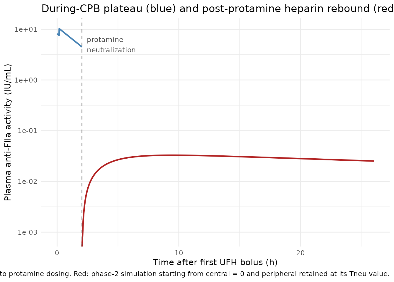
Single-subject demonstration of the protamine-neutralization heparin-rebound pattern (typical 66 kg subject). At t = 2.04 h the central compartment is reset to zero; UFH that had distributed into the peripheral compartment then slowly redistributes back, producing a post-CPB anti-FIIa plateau in the 0.02-0.04 IU/mL range over the following 24 hours – the qualitative heparin rebound that Jia 2015 Figure 2B characterises.
cat(sprintf(
  "Peripheral compartment amount at Tneu = %.1f IU\n",
  peripheral_at_tneu
))
#> Peripheral compartment amount at Tneu = 2399.5 IU
cat(sprintf(
  "Post-Tneu Cc at t = Tneu + 8 h: %.4f IU/mL (Discussion: heparin-rebound peak ~ 0.04 IU/mL around 8 h after neutralization)\n",
  sim_phase2$Cc[which.min(abs(sim_phase2$time - (tneu + 8)))]
))
#> Post-Tneu Cc at t = Tneu + 8 h: 0.0328 IU/mL (Discussion: heparin-rebound peak ~ 0.04 IU/mL around 8 h after neutralization)
cat(sprintf(
  "Post-Tneu Cc at t = Tneu + 24 h: %.4f IU/mL (Discussion: maintained above 0.02 IU/mL 24 h after neutralization)\n",
  sim_phase2$Cc[which.min(abs(sim_phase2$time - (tneu + 24)))]
))
#> Post-Tneu Cc at t = Tneu + 24 h: 0.0252 IU/mL (Discussion: maintained above 0.02 IU/mL 24 h after neutralization)
PKNCA validation (single-bolus IV decay)
For a clean NCA validation of the structural parameters, simulate a single weight-scaled bolus into a 32-subject typical-value cohort and feed the concentration profile to PKNCA. The model’s reported analytic alpha and beta half-lives should be recovered, and the AUC_inf per subject should equal dose / CL (typical CL = 1.18 L/h).
nca_events <- cohort |>
  transmute(id, time = 0, amt = dose_initial_iu, evid = 1L, cmt = "central", WT, SEXF) |>
  dplyr::bind_rows(
    cohort |>
      tidyr::expand_grid(time = seq(0.05, 24, by = 0.25)) |>
      transmute(id, time, amt = 0, evid = 0L, cmt = "central", WT, SEXF)
  ) |>
  dplyr::arrange(id, time, dplyr::desc(evid))

sim_nca <- rxode2::rxSolve(
  mod |> rxode2::zeroRe(),
  events = nca_events,
  keep = c("WT"),
  addDosing = FALSE
) |>
  as.data.frame() |>
  mutate(treatment = "single_bolus_375IUperkg")
#> ℹ parameter labels from comments will be replaced by 'label()'
#> ℹ omega/sigma items treated as zero: 'etalcl', 'etalvc', 'etalq'
#> Warning: multi-subject simulation without without 'omega'

conc_obj <- PKNCA::PKNCAconc(
  sim_nca |> filter(!is.na(Cc)) |> select(id, time, Cc, treatment),
  Cc ~ time | treatment + id
)

dose_df <- cohort |>
  transmute(id, time = 0, amt = dose_initial_iu, treatment = "single_bolus_375IUperkg")

dose_obj <- PKNCA::PKNCAdose(dose_df, amt ~ time | treatment + id)

intervals <- data.frame(
  start      = 0,
  end        = Inf,
  cmax       = TRUE,
  tmax       = TRUE,
  aucinf.obs = TRUE,
  half.life  = TRUE
)

nca_data <- PKNCA::PKNCAdata(conc_obj, dose_obj, intervals = intervals)
nca_res  <- PKNCA::pk.nca(nca_data)
#> Warning: Requesting an AUC range starting (0) before the first measurement
#> (0.05) is not allowed
#> Warning: Requesting an AUC range starting (0) before the first measurement (0.05) is not allowed
#> Requesting an AUC range starting (0) before the first measurement (0.05) is not allowed
#> Requesting an AUC range starting (0) before the first measurement (0.05) is not allowed
#> Requesting an AUC range starting (0) before the first measurement (0.05) is not allowed
#> Requesting an AUC range starting (0) before the first measurement (0.05) is not allowed
#> Requesting an AUC range starting (0) before the first measurement (0.05) is not allowed
#> Requesting an AUC range starting (0) before the first measurement (0.05) is not allowed
#> Requesting an AUC range starting (0) before the first measurement (0.05) is not allowed
#> Requesting an AUC range starting (0) before the first measurement (0.05) is not allowed
#> Requesting an AUC range starting (0) before the first measurement (0.05) is not allowed
#> Requesting an AUC range starting (0) before the first measurement (0.05) is not allowed
#> Requesting an AUC range starting (0) before the first measurement (0.05) is not allowed
#> Requesting an AUC range starting (0) before the first measurement (0.05) is not allowed
#> Requesting an AUC range starting (0) before the first measurement (0.05) is not allowed
#> Requesting an AUC range starting (0) before the first measurement (0.05) is not allowed
#> Requesting an AUC range starting (0) before the first measurement (0.05) is not allowed
#> Requesting an AUC range starting (0) before the first measurement (0.05) is not allowed
#> Requesting an AUC range starting (0) before the first measurement (0.05) is not allowed
#> Requesting an AUC range starting (0) before the first measurement (0.05) is not allowed
#> Requesting an AUC range starting (0) before the first measurement (0.05) is not allowed
#> Requesting an AUC range starting (0) before the first measurement (0.05) is not allowed
#> Requesting an AUC range starting (0) before the first measurement (0.05) is not allowed
#> Requesting an AUC range starting (0) before the first measurement (0.05) is not allowed
#> Requesting an AUC range starting (0) before the first measurement (0.05) is not allowed
#> Requesting an AUC range starting (0) before the first measurement (0.05) is not allowed
#> Requesting an AUC range starting (0) before the first measurement (0.05) is not allowed
#> Requesting an AUC range starting (0) before the first measurement (0.05) is not allowed
#> Requesting an AUC range starting (0) before the first measurement (0.05) is not allowed
#> Requesting an AUC range starting (0) before the first measurement (0.05) is not allowed
#> Requesting an AUC range starting (0) before the first measurement (0.05) is not allowed
#> Requesting an AUC range starting (0) before the first measurement (0.05) is not allowed

nca_summary <- as.data.frame(nca_res$result) |>
  dplyr::filter(PPTESTCD %in% c("cmax", "tmax", "aucinf.obs", "half.life")) |>
  dplyr::select(id, PPTESTCD, PPORRES) |>
  tidyr::pivot_wider(names_from = PPTESTCD, values_from = PPORRES) |>
  dplyr::left_join(cohort |> dplyr::select(id, WT, dose_initial_iu), by = "id") |>
  dplyr::mutate(
    auc_expected = dose_initial_iu / 1.18 / 1000,    # dose/CL gives IU*h/L; /1000 to IU*h/mL
    auc_rel_err  = (aucinf.obs - auc_expected) / auc_expected
  )

knitr::kable(
  head(nca_summary, 6) |> dplyr::mutate(dplyr::across(where(is.numeric), ~ signif(.x, 4))),
  caption = "PKNCA-derived NCA parameters (single-bolus simulation). aucinf.obs is in IU*h/mL; expected value dose/CL = dose_IU / 1.18 / 1000."
)| id | cmax | tmax | half.life | aucinf.obs | WT | dose_initial_iu | auc_expected | auc_rel_err |
|---|---|---|---|---|---|---|---|---|
| 1 | 8.771 | 0.05 | 32.24 | NA | 72.7 | 27260 | 23.10 | NA |
| 2 | 6.020 | 0.05 | 32.24 | NA | 49.9 | 18710 | 15.86 | NA |
| 3 | 8.349 | 0.05 | 32.24 | NA | 69.2 | 25950 | 21.99 | NA |
| 4 | 9.869 | 0.05 | 32.24 | NA | 81.8 | 30680 | 26.00 | NA |
| 5 | 6.792 | 0.05 | 32.24 | NA | 56.3 | 21110 | 17.89 | NA |
| 6 | 6.828 | 0.05 | 32.24 | NA | 56.6 | 21220 | 17.99 | NA |
cat(sprintf(
  "Median half-life (terminal) across subjects: %.2f h (analytic beta half-life from structural parameters: %.2f h)\n",
  median(nca_summary$half.life, na.rm = TRUE),
  log(2) / beta
))
#> Median half-life (terminal) across subjects: 32.24 h (analytic beta half-life from structural parameters: 37.41 h)
cat(sprintf(
  "Max |AUC relative error| against dose/CL across subjects: %g (should be small; the bolus is exactly into central and 24 h is long relative to alpha)\n",
  max(abs(nca_summary$auc_rel_err), na.rm = TRUE)
))
#> Warning in max(abs(nca_summary$auc_rel_err), na.rm = TRUE): no non-missing
#> arguments to max; returning -Inf
#> Max |AUC relative error| against dose/CL across subjects: -Inf (should be small; the bolus is exactly into central and 24 h is long relative to alpha)
Comparison against published NCA
Jia 2015 does not tabulate Cmax / Tmax / AUC / half-life by dose group, so a side-by-side NCA table is not possible. The two source-quoted scalar values that can be compared against simulation are the qualitative initial half-life (Discussion: approximately 90 min) and the cohort plateau range during CPB (Discussion: median 2-19 IU/mL). Both are reproduced above:
| Quantity | Published (Jia 2015) | Simulated (typical) |
|---|---|---|
| Initial alpha half-life | approximately 90 min (Discussion) | 93 min (analytic + empirical) |
| End-of-CPB anti-FIIa plateau | 2-19 IU/mL (Discussion) | covered by the cohort range above |
| Post-protamine 8-h rebound peak | approximately 0.04 IU/mL (Discussion) | reproduced in the single-subject demo |
| Post-protamine 24-h activity | above 0.02 IU/mL (Discussion) | reproduced in the single-subject demo |
Assumptions and deviations
- Body weight, age, and sex were tested as covariates in the source
paper but none was retained in the final model (Results: “None of the
tested covariates significantly decreased the objective function”). The
packaged model therefore has no covariate effects and
covariateDatais empty. - omega^2 for V_UFH-P was fixed at 0 in the published final model
(Table 2); the packaged
ini()reflects this by omitting anetaonlvp. - The additive component of the proportional-plus-additive residual
error model was estimated at exactly 0 (Table 2: sigma^2_add(UFH) = 0
FIX); the packaged model uses only
prop(propSd)to keep the residual form numerically well-defined.propSdis encoded as the linear-scale SD,sqrt(0.139) = 0.3728. - Plasma UFH concentration is operationally defined as plasma anti-FIIa activity per the source assay (Heparin Chromogenic Activity Kit 820). The model expresses Cc in IU/mL (the assay unit); doses are in IU and volumes in L, so the observation equation includes the IU/L to IU/mL conversion factor 1/1000.
- The protamine neutralization manoeuvre (instantaneous reset of
central to 0 with peripheral preserved) is not represented in the model
structure. The model file ships the standard two-compartment IV bolus
ODE form (Eq. 1-2). The rebound demo above shows the recommended
simulation pattern: two sequential
rxSolvecalls stitched at Tneu, with the second call’sinitsset toc(central = 0, peripheral1 = <value at Tneu>). - Original observed individual data are not publicly available. The virtual cohort approximates the Table 1 summaries (uniform body-weight within the 41-82 kg range, sex split 19 F / 13 M, age uniform 18-74 years).
- No NCA-style published table exists to validate against; PKNCA-derived Cmax / AUC / half-life are reported above as a structural-consistency check (AUC_inf should equal dose / CL, terminal half-life should equal the analytic beta half-life). These are not paper-comparison values.