Rozanolixizumab anti-FcRn PK/PD, monkey to human (Lledo-Garcia 2022)
Source:vignettes/articles/LledoGarcia_2022_rozanolixizumab.Rmd
LledoGarcia_2022_rozanolixizumab.RmdModel and source
Rozanolixizumab is a humanized IgG4P monoclonal antibody against the human neonatal Fc receptor (FcRn). By occupying FcRn it blocks the salvage pathway that normally recycles endogenous IgG, so circulating IgG (including pathogenic autoantibodies) is diverted to lysosomal degradation. Lledo-Garcia 2022 builds a semi-mechanistic PK/PD model of that system in cynomolgus monkey, translates it to human by allometry to design the first-in-human (FIH) study, and then re-estimates it against the FIH data.
The paper therefore reports three distinct parameter sets for one structure, and this package ships each as its own model file (the author’s structure is reproduced rather than collapsed):
| Model | What it is | Source |
|---|---|---|
LledoGarcia_2022_rozanolixizumab_cyno |
Fitted to single-dose IV cynomolgus monkey data | Table 1, first value column |
LledoGarcia_2022_rozanolixizumab_translated |
Allometric forward projection to a 75 kg human; used to design the FIH study, before any human data existed | Table 1, second value column |
LledoGarcia_2022_rozanolixizumab |
Final model, re-estimated against the FIH IV cohorts | Table 2, FIH-estimated column |
mods <- lapply(
  c(cyno       = "LledoGarcia_2022_rozanolixizumab_cyno",
    translated = "LledoGarcia_2022_rozanolixizumab_translated",
    final      = "LledoGarcia_2022_rozanolixizumab"),
  function(nm) rxode2::rxode(readModelDb(nm))
)
#> ℹ parameter labels from comments will be replaced by 'label()'
#> ℹ parameter labels from comments will be replaced by 'label()'- Citation: Lledo-Garcia R, Dixon K, Shock A, Oliver R. Pharmacokinetic-pharmacodynamic modelling of the anti-FcRn monoclonal antibody rozanolixizumab: Translation from preclinical stages to the clinic. CPT Pharmacometrics Syst Pharmacol. 2022;11(1):116-128. doi:10.1002/psp4.12739
- Article: https://doi.org/10.1002/psp4.12739
- Supplement (Texts S1-S4, Figures S1-S2): https://doi.org/10.1002/psp4.12739, “Supporting Information”
Population
The cynomolgus model was fitted to single-dose IV data at 5, 10 and 30 mg/kg. The underlying animal study is Smith et al. 2018 (mAbs 10:1111-1130; reference 9 of the source paper), which used four healthy young adult male animals per dosing group weighing at least 2.3 kg and aged roughly 135-185 weeks, so the three single-dose IV groups contribute 12 animals. Multiple-dose data collected before antidrug antibodies were detected were held back for external validation.
The final human model was fitted to the IV cohorts of the FIH study NCT02220153 (Kiessling et al. 2017, Sci Transl Med 9:eaan1208; reference 11). That study randomised 49 healthy subjects to rozanolixizumab (n = 36) or placebo (n = 13) across six cohorts; the first three were IV at 1, 4 and 7 mg/kg with n = 6 each, and Lledo-Garcia 2022 analysed only the IV cohorts. Dose escalation was stopped at 7 mg/kg on tolerability grounds, so the model sees a narrower dose range than planned. Lledo-Garcia 2022 does not tabulate baseline demographics for this cohort.
The same information is available programmatically from each model’s
population metadata.
str(mods$final$population, max.level = 1)
#> List of 6
#>  $ species      : chr "human"
#>  $ n_subjects   : int 18
#>  $ n_studies    : int 1
#>  $ disease_state: chr "healthy adult volunteers"
#>  $ dose_range   : chr "1, 4 and 7 mg/kg single intravenous infusion (6 subjects per dose cohort)"
#>  $ notes        : chr "First-in-human study NCT02220153 (Kiessling et al. 2017 Sci Transl Med 9:eaan1208; reference 11 of the source p"| __truncated__
Model structure
The structure is identical across all three parameter sets: a two-compartment target-mediated disposition (TMDD) model under the quasi-equilibrium approximation, coupled to an indirect-response model in which free drug stimulates IgG catabolism. Figure 1 of the paper is the schematic.
Two structural simplifications are load-bearing (Methods, and Supplementary Text S1):
- FcRn is highly expressed on vascular endothelium, so the endosomal compartment is lumped with the central compartment and binding is assumed to equilibrate instantly.
- Rozanolixizumab binds FcRn through its Fab, and the clearance of
free FcRn equals the clearance of the drug:FcRn complex (both
CLB). Because those two are equal, the total FcRn pool is constant in time, so the paper carries no differential equation for it –TBenters the binding quadratic as a constant.
Supplementary Text S1 and S2 give the equations (recovered from the MathType objects embedded in the supplement’s Word file):
dTA/dt    = -FA(t)*CLA/V - CPLX(t)*CLB/V - Q*FA(t)/V + Q*APERI(t)/V2 + input
dAPERI/dt =  Q*FA(t)/V - Q*APERI(t)/V2

CPLX  = ( (KD*V + TA(t) + TB) - sqrt( (KD*V + TA(t) + TB)^2 - 4*TA(t)*TB ) ) / 2
FA    = TA - CPLX
CLB   = KDEG*V ;  RB = CFCRN*KDEG*V ;  TB = V*RB/CLB

EFF     = EMAX*FAC(t) / (FAC(t) + EC50)      with FAC = MWT*FA/V
dIGG/dt = IGSS*KOUT - KOUT*IGG(t)*(1 + EFF)
The packaged model divides the amount-scale binding quadratic through
by V, which is an algebraic identity (the expression is
homogeneous of degree one), so that drug and target are carried on a
single mg/L (= ug/mL) scale with dosing in mg. The free-drug root is
written in the numerically stable arrangement
cfree = (disc + sqrt(disc^2 + 4*kd*ctot))/2.
mods$final$funTxt
#> [1] "mwt <- 148000\nnm2mgl <- mwt/1e+06\nvc <- exp(lvc + etalvc)\nq <- exp(lq)\nvp <- exp(lvp)\ncl <- exp(lcl)\nkdeg <- exp(lkdeg + etalkdeg)\nkd <- exp(lkd) * nm2mgl\nrtot <- exp(lrtot) * nm2mgl\nclb <- kdeg * vc\nrbase <- exp(lrbase + etalrbase)\nkout <- exp(lkout)\nemax <- exp(lemax)\nec50 <- exp(lec50)\nctot <- central/vc\ndisc <- ctot - rtot - kd\ncfree <- 0.5 * (disc + sqrt(disc * disc + 4 * kd * ctot))\ncplx <- ctot - cfree\nd/dt(central) <- -cl * cfree - clb * cplx - q * cfree + (q/vp) * peripheral1\nd/dt(peripheral1) <- q * cfree - (q/vp) * peripheral1\neff <- emax * cfree/(cfree + ec50)\ntotal_igg(0) <- rbase\nd/dt(total_igg) <- rbase * kout - kout * total_igg * (1 + eff)\nrb <- exp(lrtot) * kdeg * vc\nCtot <- ctot\npctChangeIgG <- 100 * (total_igg - rbase)/rbase\nCc <- cfree\nIgG_obs <- total_igg\nCc ~ prop(propSd)\nIgG_obs ~ prop(propSd_IgG_obs)"
Source trace
Per-parameter provenance is recorded as an in-file comment beside
each ini() entry. Collected here for review:
| Quantity | cyno | translated | final (FIH) | Source |
|---|---|---|---|---|
V (L) |
0.108 | 2.55 | 2.7 | Table 1 / Table 2 |
Q (L/day) |
0.0221 | 0.237 | 0.271 | Table 1 / Table 2 |
V2 (L) |
0.0162 | 0.383 | 0.36 | Table 1 / Table 2 |
CLA (L/day) |
0.0709 | 0.7605 | 0.968 | Table 1 / Table 2 |
KD (nmol/L) |
0.827 | 0.359 | 1 | Table 1 / Table 2 |
[FcRn] (nmol/L) |
592.89 | 592.89 | 147 | Table 1 / Table 2 |
Kdeg (1/day) |
0.3389 | 0.277 | 0.88 | Table 1 / Table 2 |
IgG base (g/L) |
10.5 | 11.65 | 9.88 | Table 1 / Table 2 |
Kout (1/day) |
0.0431 | 0.031 | 0.0364 | Table 1 / Table 2 |
Emax |
7.58 | 7.58 | 4.24 | Table 1 / Table 2 |
EC50 (mg/L) |
1.14 | 0.4959 | 0.154 | Table 1 / Table 2 |
| IIV (CV%) | not reported | V 16.35, V2 28.75, CLA 35.15, Kdeg 18, IgG base 21, Kout 22, Emax 25, EC50 58 | V 15.8, Kdeg 30.3, IgG base 18.4 | Table 1 / Table 2 |
| Proportional RUV | not reported | not reported | PK 9.3%, IgG 5.8% | Table 2 |
| PK / PD equations | Supplementary Text S1 / S2 | supplement | ||
| Allometry | Supplementary Text S4 | supplement | ||
MWT = 148 kDa |
not in the paper – RYSTIGGO US prescribing information section 11 | see Errata |
Gate 1: the derived-quantity identities
Table 1 and Table 2 print CLB and RB as
derived quantities (Table 2 footnote b: “Derived value (not
estimated)”), with RB = [FcRn]*Kdeg*V and
CLB = Kdeg*V. The packaged models compute both from their
primaries, so reproducing the printed numbers is an exact, deterministic
check on the volume, the target concentration and the degradation rate
all at once – no seed, no cohort, no solver tolerance involved.
one_obs <- function(mod, dose_mg) {
  ev <- rbind(
    data.frame(id = 1L, time = 0, amt = dose_mg, evid = 1L,
               cmt = "central", dvid = NA_integer_),
    data.frame(id = 1L, time = c(0, 1), amt = NA_real_, evid = 0L,
               cmt = "central", dvid = 1L)
  )
  as.data.frame(rxode2::rxSolve(rxode2::zeroRe(mod), ev, returnType = "data.frame"))
}

derived <- tibble::tibble(
  Model     = c("cyno", "translated", "final"),
  RB_model  = vapply(mods, function(m) one_obs(m, 1)$rb[1], numeric(1)),
  RB_paper  = c(21.7, 419.748, 349.3)
) |>
  mutate(pct_diff = 100 * (RB_model - RB_paper) / RB_paper)
#> Warning: No omega parameters in the model
#> ℹ omega/sigma items treated as zero: 'etalvc', 'etalvp', 'etalcl', 'etalkdeg', 'etalrbase', 'etalkout', 'etalemax', 'etalec50'
#> ℹ omega/sigma items treated as zero: 'etalvc', 'etalkdeg', 'etalrbase'

derived |>
  rename("RB, model (nmol/day)" = RB_model,
         "RB, paper (nmol/day)" = RB_paper,
         "Difference (%)"       = pct_diff) |>
  knitr::kable(digits = c(0, 2, 3, 3),
caption = "RB = [FcRn] x Kdeg x V reproduced from the packaged primaries.")| Model | RB, model (nmol/day) | RB, paper (nmol/day) | Difference (%) |
|---|---|---|---|
| cyno | 21.70 | 21.700 | 0.002 |
| translated | 418.79 | 419.748 | -0.229 |
| final | 349.27 | 349.300 | -0.008 |
Gate 2: the translated model reproduces Figure 3a
Figure 3a overlays the translated model’s predictions on the observed FIH concentrations, and its y axis is labelled “Free drug concentration (ug/mL)”. That label is what settles an otherwise ambiguous modelling choice: the PK observation is the free drug concentration, not total. It is also a sharp quantitative test, because free and total differ by orders of magnitude at the low dose where FcRn is far from saturated.
peak_free <- function(mod, dose_mg) {
  s <- one_obs(mod, dose_mg)
  c(free = s$Cc[1], total = s$Ctot[1])
}

fig3a <- tibble::tibble(dose_mgkg = c(1, 4, 7)) |>
  rowwise() |>
  mutate(pk = list(peak_free(mods$translated, dose_mgkg * 75))) |>
  ungroup() |>
  mutate(free_ugmL  = vapply(pk, function(x) x[["free"]],  numeric(1)),
         total_ugmL = vapply(pk, function(x) x[["total"]], numeric(1))) |>
  select(-pk)
#> ℹ omega/sigma items treated as zero: 'etalvc', 'etalvp', 'etalcl', 'etalkdeg', 'etalrbase', 'etalkout', 'etalemax', 'etalec50'
#> ℹ omega/sigma items treated as zero: 'etalvc', 'etalvp', 'etalcl', 'etalkdeg', 'etalrbase', 'etalkout', 'etalemax', 'etalec50'
#> ℹ omega/sigma items treated as zero: 'etalvc', 'etalvp', 'etalcl', 'etalkdeg', 'etalrbase', 'etalkout', 'etalemax', 'etalec50'

fig3a |>
  rename("Dose (mg/kg)"          = dose_mgkg,
         "Peak FREE (ug/mL)"     = free_ugmL,
         "Peak TOTAL (ug/mL)"    = total_ugmL) |>
  knitr::kable(digits = c(0, 4, 1),
caption = "Translated model, peak concentration after a single IV dose.")| Dose (mg/kg) | Peak FREE (ug/mL) | Peak TOTAL (ug/mL) |
|---|---|---|
| 1 | 0.0268 | 29.4 |
| 4 | 30.0542 | 117.6 |
| 7 | 118.1741 | 205.9 |
Reading the model medians off Figure 3a gives roughly 0.02, 20-30 and 150 ug/mL at 1, 4 and 7 mg/kg. The free-drug column matches all three; the total-drug column is wrong by a factor of about 1100 at 1 mg/kg and about 4 at 4 mg/kg. This is the check that pins the observation variable.
stopifnot(
  # 1 mg/kg: deeply target-bound, free drug is a small fraction of total.
  fig3a$free_ugmL[1] > 0.01, fig3a$free_ugmL[1] < 0.05,
  # 4 mg/kg: FcRn just saturating.
  fig3a$free_ugmL[2] > 20,   fig3a$free_ugmL[2] < 40,
  # 7 mg/kg: well past saturation.
  fig3a$free_ugmL[3] > 100,  fig3a$free_ugmL[3] < 150,
  # The total-drug reading is excluded by the same figure.
  fig3a$total_ugmL[1] > 25
)
Gate 3: the final model reproduces the observed IgG reductions
The Results section reports the FIH outcome directly: “mean reductions in IgG of 14.5, 33.4, and 47.6% (10 days postdose) were observed for the 1, 4, and 7 mg/kg rozanolixizumab doses”. The prediction-corrected VPCs of Figure 4 confirm the final model described these data. Because these are the paper’s own headline numbers and the final model was fitted to them, reproducing them from the packaged typical-value parameters exercises the whole chain: the binding quadratic, the unit conversion through the molecular weight, and the indirect-response PD.
igg_profile <- function(mod, dose_mg, tmax = 84) {
  tt <- sort(unique(c(seq(0, 2, by = 0.05), seq(2, 14, by = 0.25),
                      seq(14, tmax, by = 1))))
  ev <- rbind(
    data.frame(id = 1L, time = 0, amt = dose_mg, evid = 1L,
               cmt = "central", dvid = NA_integer_),
    data.frame(id = 1L, time = tt, amt = NA_real_, evid = 0L,
               cmt = "central", dvid = 1L)
  )
  as.data.frame(rxode2::rxSolve(rxode2::zeroRe(mod), ev, returnType = "data.frame"))
}

day10 <- lapply(c(1, 4, 7), function(d) {
  s <- igg_profile(mods$final, d * 75, tmax = 20)
  tibble::tibble(dose_mgkg = d,
                 model_pct = -s$pctChangeIgG[which.min(abs(s$time - 10))])
}) |>
  bind_rows() |>
  mutate(observed_pct = c(14.5, 33.4, 47.6),
         diff_pp      = model_pct - observed_pct)
#> ℹ omega/sigma items treated as zero: 'etalvc', 'etalkdeg', 'etalrbase'
#> ℹ omega/sigma items treated as zero: 'etalvc', 'etalkdeg', 'etalrbase'
#> ℹ omega/sigma items treated as zero: 'etalvc', 'etalkdeg', 'etalrbase'

day10 |>
  rename("Dose (mg/kg)"                 = dose_mgkg,
         "Model IgG reduction (%)"      = model_pct,
         "Observed IgG reduction (%)"   = observed_pct,
         "Difference (percentage pts)"  = diff_pp) |>
  knitr::kable(digits = c(0, 1, 1, 1),
caption = "Day-10 IgG reduction, final model typical value vs the observed FIH means (Results).")| Dose (mg/kg) | Model IgG reduction (%) | Observed IgG reduction (%) | Difference (percentage pts) |
|---|---|---|---|
| 1 | 14.1 | 14.5 | -0.4 |
| 4 | 34.7 | 33.4 | 1.3 |
| 7 | 44.2 | 47.6 | -3.4 |
stopifnot(
  # Every dose within 5 percentage points of the observed mean.
  all(abs(day10$diff_pp) < 5),
  # And the dose-response ordering is preserved.
  !is.unsorted(day10$model_pct)
)
Gate 4: the preclinical model spans the observed monkey response
The Discussion states that the monkey data “demonstrated 49-75%
decreases in IgG from baseline (following the rozanolixizumab dose range
studied)” of 5, 10 and 30 mg/kg. Converting mg/kg to mg needs an animal
body weight, which the paper does not report; the weight implied by its
own allometric translation (V 0.108 L to 2.55 L at exponent
1, and V2 0.0162 L to 0.383 L, both a 23.6-fold ratio
against 75 kg) is about 3.17 kg, and that is what is used here.
The gated claims are therefore the ones that are robust to that unknown: the top of the dose range reaches the paper’s upper figure, and the response is monotone in dose. The lower bound is not gated – see Errata.
bw_cyno <- 75 / (2.55 / 0.108)   # kg, implied by the paper's own allometry

cyno_nadir <- lapply(c(5, 10, 30), function(d) {
  s <- igg_profile(mods$cyno, d * bw_cyno, tmax = 60)
  tibble::tibble(dose_mgkg = d, nadir_pct = -min(s$pctChangeIgG))
}) |>
  bind_rows()
#> Warning: No omega parameters in the model
#> No omega parameters in the model
#> No omega parameters in the model

cyno_nadir |>
  rename("Dose (mg/kg)" = dose_mgkg, "Maximum IgG reduction (%)" = nadir_pct) |>
  knitr::kable(digits = 1,
               caption = paste0("Preclinical model, maximum IgG reduction at an implied ",
round(bw_cyno, 2), " kg body weight."))| Dose (mg/kg) | Maximum IgG reduction (%) |
|---|---|
| 5 | 39.1 |
| 10 | 57.9 |
| 30 | 73.7 |
stopifnot(
  # 30 mg/kg reaches the top of the observed 49-75% band.
  cyno_nadir$nadir_pct[3] > 65, cyno_nadir$nadir_pct[3] < 85,
  # Monotone dose-response, which no body-weight assumption can disturb.
  !is.unsorted(cyno_nadir$nadir_pct)
)
Virtual cohort and stochastic simulation
Original observed data are not available. The VPC-style figures below use virtual cohorts of 100 subjects per dose arm, matching the FIH IV dose levels. A 75 kg reference subject is used throughout because the models carry no body weight covariate – allometry was applied once, when translating the monkey parameters, and is not part of the model.
make_arm <- function(dose_mgkg, n = 100, id_offset = 0L, tmax = 84) {
  tt <- sort(unique(c(seq(0, 2, by = 0.1), seq(2, 14, by = 0.5),
                      seq(14, tmax, by = 2))))
  ids <- id_offset + seq_len(n)
  dose <- data.frame(id = ids, time = 0, amt = dose_mgkg * 75, evid = 1L,
                     cmt = "central", dvid = NA_integer_)
  obs <- expand.grid(id = ids, time = tt)
  obs <- data.frame(id = obs$id, time = obs$time, amt = NA_real_, evid = 0L,
                    cmt = "central", dvid = 1L)
  out <- rbind(dose, obs)
  out$treatment <- paste0(dose_mgkg, " mg/kg IV")
  out[order(out$id, out$time, -out$evid), ]
}

doses <- c(1, 4, 7)
events <- bind_rows(lapply(seq_along(doses), function(i) {
  make_arm(doses[i], n = 100, id_offset = (i - 1L) * 1000L)
}))
stopifnot(!anyDuplicated(unique(events[, c("id", "time", "evid")])))
rxSolve on an rxUi scales super-linearly
with the number of subjects in a single call, so each arm is solved
separately and the results are stacked.
solve_arm <- function(mod, ev) {
  as.data.frame(
    rxode2::rxSolve(mod, events = ev, keep = c("treatment"),
                    returnType = "data.frame")
  )
}

sim_final <- bind_rows(lapply(split(events, events$treatment), function(ev) {
  solve_arm(mods$final, ev)
}))
sim_translated <- bind_rows(lapply(split(events, events$treatment), function(ev) {
  solve_arm(mods$translated, ev)
}))
Replicate published figures
# Replicates Figure 3a of Lledo-Garcia 2022: translated-model free drug
# concentration vs time, by IV dose cohort.
sim_translated |>
  filter(time > 0, Cc > 0) |>
  group_by(treatment, time) |>
  summarise(Q05 = quantile(Cc, 0.05), Q50 = median(Cc),
            Q95 = quantile(Cc, 0.95), .groups = "drop") |>
  ggplot(aes(time, Q50)) +
  geom_ribbon(aes(ymin = Q05, ymax = Q95), alpha = 0.25, fill = "steelblue") +
  geom_line(colour = "steelblue") +
  facet_wrap(~treatment, scales = "free_y") +
  scale_y_log10() +
  coord_cartesian(xlim = c(0, 6)) +
  labs(x = "Time (days)", y = "Free drug concentration (ug/mL)",
       title = "Figure 3a - translated model, free rozanolixizumab",
       caption = "Replicates Figure 3a of Lledo-Garcia 2022. Median with 90% prediction interval.")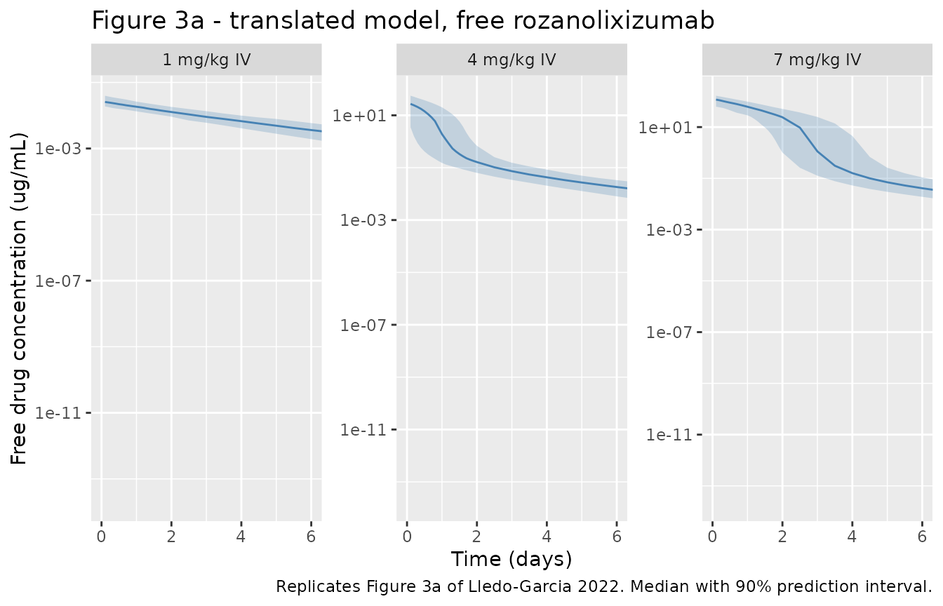
# Replicates Figure 3b of Lledo-Garcia 2022: percentage change from baseline IgG.
sim_translated |>
  filter(time > 0) |>
  group_by(treatment, time) |>
  summarise(Q05 = quantile(pctChangeIgG, 0.05), Q50 = median(pctChangeIgG),
            Q95 = quantile(pctChangeIgG, 0.95), .groups = "drop") |>
  ggplot(aes(time, Q50)) +
  geom_ribbon(aes(ymin = Q05, ymax = Q95), alpha = 0.25, fill = "darkgreen") +
  geom_line(colour = "darkgreen") +
  geom_hline(yintercept = 0, linetype = "dotted") +
  facet_wrap(~treatment) +
  labs(x = "Time (days)", y = "Change from baseline IgG (%)",
       title = "Figure 3b - translated model, IgG response",
       caption = "Replicates Figure 3b of Lledo-Garcia 2022. Median with 90% prediction interval.")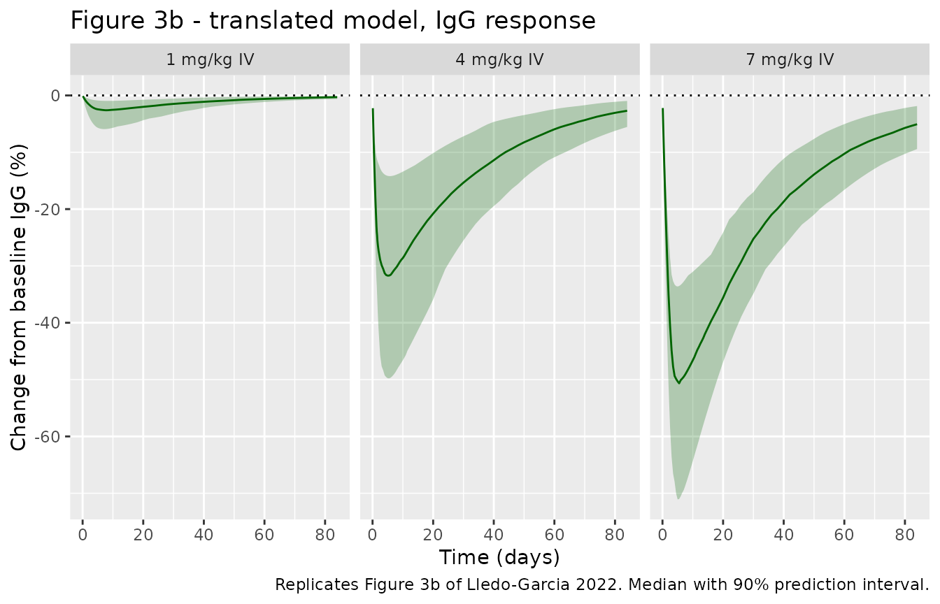
# Replicates Figure 4 of Lledo-Garcia 2022: final-model prediction-corrected VPC
# equivalent, for rozanolixizumab concentration (a) and IgG concentration (b).
bind_rows(
  sim_final |> transmute(treatment, time, value = Cc,
                         panel = "(a) Free rozanolixizumab (ug/mL)"),
  sim_final |> transmute(treatment, time, value = IgG_obs,
                         panel = "(b) Total IgG (g/L)")
) |>
  filter(time > 0, value > 0) |>
  group_by(panel, treatment, time) |>
  summarise(Q025 = quantile(value, 0.025), Q50 = median(value),
            Q975 = quantile(value, 0.975), .groups = "drop") |>
  ggplot(aes(time, Q50, colour = treatment, fill = treatment)) +
  geom_ribbon(aes(ymin = Q025, ymax = Q975), alpha = 0.2, colour = NA) +
  geom_line() +
  facet_wrap(~panel, scales = "free_y") +
  labs(x = "Time (days)", y = NULL, colour = NULL, fill = NULL,
       title = "Figure 4 - final human model",
       caption = paste("Replicates Figure 4 of Lledo-Garcia 2022.",
                       "Median with 2.5th-97.5th percentile band."))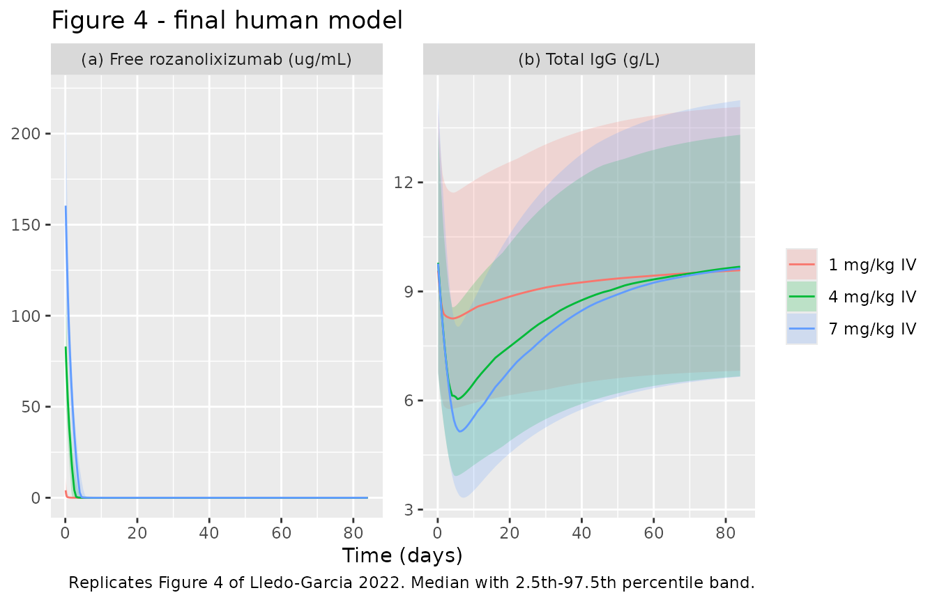
PKNCA validation
The paper’s central pharmacological claim is that the system is nonlinear at low dose and moves towards linearity as dose increases (“Prediction/observation alignment increased at higher doses, as the system moved towards linearity for both PK and IgG”; the FIH report likewise describes “nonlinear increases with dose”). That is a directly testable NCA statement: because FcRn acts as a saturable sink for free drug, dose-normalised free-drug exposure must increase with dose, and the increase must flatten out once the receptor is saturated.
The NCA window is 0-14 days. Free drug is essentially gone well before that – at 1 mg/kg the median free concentration has fallen from about 6.8 ug/mL at time zero to about 1e-6 ug/mL by day 14, so roughly 23 half-lives – and beyond about day 28 the profile decays into solver noise and drifts marginally negative (order 1e-12 ug/mL). Truncating keeps the assertion below meaningful rather than silently repairing negative values, and the omitted tail contributes nothing to AUC.
sim_nca <- sim_final |>
  filter(!is.na(Cc), time <= 14) |>
  select(id, time, Cc, treatment)

# Guarantee a time-zero row per (id, treatment) so PKNCA can anchor AUC.
sim_nca <- bind_rows(
  sim_nca,
  sim_nca |> distinct(id, treatment) |> mutate(time = 0, Cc = 0)
) |>
  distinct(id, treatment, time, .keep_all = TRUE) |>
  arrange(id, treatment, time)

# TMDD tails can drift marginally negative in the solver; PKNCA would take
# log() of those. Assert instead of silently repairing.
stopifnot(all(sim_nca$Cc >= 0))

conc_obj <- PKNCA::PKNCAconc(sim_nca, Cc ~ time | treatment + id)

dose_df <- events |>
  filter(evid == 1) |>
  select(id, time, amt, treatment)
dose_obj <- PKNCA::PKNCAdose(dose_df, amt ~ time | treatment + id)

intervals <- data.frame(start = 0, end = 14,
                        cmax = TRUE, tmax = TRUE, auclast = TRUE)

nca_res <- PKNCA::pk.nca(PKNCA::PKNCAdata(conc_obj, dose_obj,
                                          intervals = intervals))
nca_tab <- as.data.frame(nca_res) |>
  group_by(treatment, PPTESTCD) |>
  summarise(median = median(PPORRES), .groups = "drop") |>
  pivot_wider(names_from = PPTESTCD, values_from = median) |>
  mutate(dose_mg = as.numeric(sub(" mg/kg IV", "", treatment)) * 75,
         auc_per_mg  = auclast / dose_mg,
         cmax_per_mg = cmax / dose_mg) |>
  arrange(dose_mg)

nca_tab |>
  select(treatment, cmax, tmax, auclast, auc_per_mg, cmax_per_mg) |>
  rename("Dose cohort"                    = treatment,
         "Cmax (ug/mL)"                   = cmax,
         "Tmax (day)"                     = tmax,
         "AUC0-14 (ug*day/mL)"            = auclast,
         "AUC0-14 / dose (ug*day/mL/mg)"  = auc_per_mg,
         "Cmax / dose (ug/mL/mg)"         = cmax_per_mg) |>
  knitr::kable(digits = c(0, 2, 2, 1, 4, 5),
               caption = paste("Median NCA of simulated FREE rozanolixizumab,",
"final model, 100 subjects per arm."))| Dose cohort | Cmax (ug/mL) | Tmax (day) | AUC0-14 (ug*day/mL) | AUC0-14 / dose (ug*day/mL/mg) | Cmax / dose (ug/mL/mg) |
|---|---|---|---|---|---|
| 1 mg/kg IV | 6.38 | 0 | 1.4 | 0.0191 | 0.08508 |
| 4 mg/kg IV | 87.68 | 0 | 95.5 | 0.3184 | 0.29228 |
| 7 mg/kg IV | 173.06 | 0 | 255.6 | 0.4868 | 0.32964 |
# Dose-normalised exposure must rise with dose: that IS the TMDD nonlinearity.
stopifnot(
  !is.unsorted(nca_tab$auc_per_mg),
  !is.unsorted(nca_tab$cmax_per_mg),
  # The nonlinearity is large between 1 and 4 mg/kg ...
  nca_tab$auc_per_mg[2] / nca_tab$auc_per_mg[1] > 2,
  # ... and much smaller between 4 and 7 mg/kg, i.e. approaching linearity.
  nca_tab$auc_per_mg[3] / nca_tab$auc_per_mg[2] <
    nca_tab$auc_per_mg[2] / nca_tab$auc_per_mg[1]
)
Comparison against published NCA
Lledo-Garcia 2022 reports no NCA table – neither Cmax, Tmax, AUC nor half-life is tabulated for either species, so there is nothing to place side by side with the simulated values above. The quantitative comparisons against published numbers in this vignette are therefore Gates 1-4, which use the paper’s derived-parameter identities (Table 1, Table 2 footnote b), its Figure 3a concentrations and its Results-section IgG reductions instead.
Assumptions and deviations
Errata and inconsistencies found in the source
-
Table 2 misprints the translated
Kdegas 0.227 /day. Table 1 gives 0.277 /day, and both derived quantities printed alongside it confirm Table 1:CLB = Kdeg*Vrequires 0.7079 / 2.55 = 0.2776, andRB = [FcRn]*Kdeg*Vrequires 419.748 / (592.89 x 2.55) = 0.2776. The packaged translated model uses 0.277. -
Table 1 and Table 2 disagree on the translated
Q(0.237 vs 0.27 L/day). Table 1’s value is the allometrically consistent one (0.0221 x (2.55/0.108)^0.75 = 0.2367) and Table 1 is the table the paper describes as the input to the simulations, so 0.237 is used. - Figure 3’s panel labels are transposed between the caption and the figure. The caption says “(a) percentage change from baseline in IgG … and (b) rozanolixizumab concentration”; the rendered figure has concentration in (a) and IgG in (b). This vignette follows the figure.
-
Supplementary Text S2 gives
IGSSin mg/L while Tables 1 and 2 print IgG baseline in mg/mL (10.5, 11.65, 9.88 – physiologically the mg/mL reading is the correct one for serum IgG). The IgG differential equation is homogeneous of degree one in IgG, so the choice of scale cannot affect any prediction; the models carry IgG in g/L (= mg/mL) as printed in the tables.
Non-paper-derived parameter values
-
MWT= 148 kDa (rozanolixizumab molecular weight). This value is not reported in any available source for this paper: not in the main text, not in Supplementary Texts S1-S4, and not in the cited characterisation paper (Smith et al. 2018, mAbs 10:1111-1130), which was retrieved and searched. It is nonetheless load-bearing, because the paper reportsKDand[FcRn]in nmol/L butEC50and all observed concentrations in mg/L, so exactly one molar-to-mass conversion is needed to put drug and target on a common scale in the binding quadratic. The value used is from the RYSTIGGO (rozanolixizumab-noli) US prescribing information, section 11 DESCRIPTION: “Rozanolixizumab-noli has an approximate molecular weight of 148 kDa” (DailyMed SPL setid 3c0eb8c2-c042-4954-b451-3baa77f5e6d1). It is hardcoded inmodel()as a unit conversion rather than declared inini(), following theSaid_2025_imatinibprecedent for molecular-weight conversion factors. Gate 2 above is an independent check on it: the free concentrations the packaged model produces at 1, 4 and 7 mg/kg agree with Figure 3a, which they would not if the conversion were materially wrong.
Modelling assumptions
-
The PK observation is free, not total, drug. The
paper never states this in prose. It is established here by the y-axis
label of Figure 3a (“Free drug concentration (ug/mL)”), corroborated by
Gate 2, and consistent with the bioanalytical method: Smith et al. 2018
describe an assay in which rozanolixizumab is captured on immobilised
FcRn, i.e. one that reports FcRn-binding-competent drug. Total drug is
still available from the packaged models as the derived variable
Ctot. -
Residual error is encoded as
fixed(0)in the cynomolgus and translated models. Table 2 prints “-” for both proportional-RUV rows of the translated column, and no RUV magnitude is reported for the monkey fit; the translated model was used for simulation rather than fitted. No value was invented. - The cynomolgus model carries no IIV. Table 1’s “IIV human (CV %)” column describes the human translation, not the monkey fit, and no monkey IIV is reported anywhere. The model is therefore a typical-value mechanism.
- The cynomolgus body weight is not reported. Only “a minimum of 2.3 kg” appears in Smith et al. 2018. Gate 4 uses 3.17 kg, the weight implied by the paper’s own allometric translation. The predicted IgG nadir at 5 mg/kg is sensitive to this choice (39% at 3.17 kg, 50% at 4.5 kg) whereas the 30 mg/kg nadir is not (74% to 77% across the same range). Gate 4 therefore asserts on the 30 mg/kg endpoint and on dose-monotonicity, and deliberately does not assert the lower edge of the paper’s observed 49-75% band. The body weight was not tuned to make that band fit.
-
Q, V2, KD and [FcRn] in the final model are estimates, not
fixed values. Table 2 footnote a marks them as “estimated with
prior information” (NONMEM NWPRIOR) and each carries an RSE, so none is
wrapped in
fixed(). -
units$dosingis mg andunits$concentrationis ug/mL. The conventions checker notes the magnitude difference; it is correct here because an amount in mg divided by a volume in L gives mg/L, which is numerically identical to ug/mL. No scaling factor is needed or applied. - The 1 mg/kg dose is known to be underpredicted. The paper says so explicitly for both the translated and the final model, and attributes it to the estimated FcRn concentration having greater leverage at low dose, with no monkey data below 5 mg/kg to inform the nonlinear region. This is a property of the published model, faithfully reproduced, not an extraction defect.