Clarithromycin (Shah 2025)
Source:vignettes/articles/Shah_2025_clarithromycin.Rmd
Shah_2025_clarithromycin.RmdModel and source
#> ℹ parameter labels from comments will be replaced by 'label()'Citation: Shah RV, Kipper K, Baker EH, Barker CIS, Oldfield I, Davidson HC, Swire CC, Philips BJ, Johnston A, Rhodes A, Sharland M, Standing JF, Lonsdale DO (2025). Intravenous Clarithromycin in Critically Ill Adults: A Population Pharmacokinetic Study. Antibiotics 14(6):559. doi:10.3390/antibiotics14060559.
Description: Two-compartment intravenous population PK model for clarithromycin in critically ill adults, with a priori allometric body-weight scaling on all disposition parameters. No covariate effects were retained and no auto-inhibition of clearance was detectable in this population.
This is the first published description of intravenous clarithromycin pharmacokinetics in humans. Clarithromycin PK had previously been described only after oral or enteral administration in humans, and intravenously only in foals.
Population
The model was fit to 121 plasma samples from 19 critically ill adults admitted to the intensive care unit at St George’s Hospital, London, all of whom received intravenous clarithromycin 500 mg every 12 h (Shah 2025 Table 1, Section 2.1). Sampling was opportunistic around the indicative schedule of Table 3, with a maximum of eight samples per participant; not every participant had a peak concentration measured. Participants were a median of 66 years old (IQR 56.7-72.7), weighed a median of 80 kg (IQR 65-95, range 53-120), and 12 of 19 were male. The cohort was severely ill: median APACHE II 20 points, 12 of 19 on vasopressors, 12 with periods of invasive ventilation, and median serum albumin of 25 g/L. Six of 19 participants had died by 90 days.
Of the 139 samples originally collected from 22 participants, 18 samples from 5 participants were excluded a priori because they were drawn during periods of renal replacement therapy (Section 2.1 and Section 4). The packaged model is therefore valid only off renal replacement therapy and must not be used to predict exposure during RRT.
The same information is available programmatically via the model’s
population metadata:
str(ui$population)
#> List of 20
#>  $ species         : chr "human"
#>  $ n_subjects      : num 19
#>  $ n_studies       : num 1
#>  $ n_samples       : num 121
#>  $ age_range       : chr "25-85.8 years"
#>  $ age_median      : chr "66 years"
#>  $ weight_range    : chr "53-120 kg"
#>  $ weight_median   : chr "80 kg"
#>  $ height_range    : chr "150-192 cm"
#>  $ height_median   : chr "173 cm"
#>  $ sex_female_pct  : num 36.8
#>  $ race_ethnicity  : Named num [1:4] 63.2 5.3 5.3 26.3
#>   ..- attr(*, "names")= chr [1:4] "White" "Black British" "Asian" "Not stated"
#>  $ disease_state   : chr "Critical illness requiring intensive care. Infection sources were chest (14), ear/nose/throat (2), skin (1), ce"| __truncated__
#>  $ dose_range      : chr "500 mg IV every 12 h (all participants)"
#>  $ regions         : chr "United Kingdom (single centre: St George's Hospital, London)"
#>  $ renal_function  : chr "Serum creatinine median 89 umol/L (IQR 71-121, range 40-276). Periods of renal replacement therapy were exclude"| __truncated__
#>  $ hepatic_function: chr "ALT median 34 U/L (IQR 24-48, range 9-166)"
#>  $ severity        : chr "APACHE II median 20 points (IQR 16-23, range 0-28); 12 participants received vasopressors; 12 had periods of in"| __truncated__
#>  $ co_medication   : chr "Concomitant drugs were screened against the British National Formulary; none was predicted to affect clarithrom"| __truncated__
#>  $ notes           : chr "Sub-study of the ABDose observational antibiotic PK/PD study (REC 14/LO/1999), the same study that supplied mod"| __truncated__
Source trace
The per-parameter origin is recorded as an in-file comment next to
each ini() entry in
inst/modeldb/specificDrugs/Shah_2025_clarithromycin.R. The
table below collects them in one place for review.
| Parameter | Value | Source |
|---|---|---|
lcl (CL) |
8.17 L/h/70 kg | Table 2, theta_CL (17% RSE) |
lvc (V1) |
25.7 L/70 kg | Table 2, theta_V1 (29% RSE) |
lq (Q) |
62.0 L/h/70 kg | Table 2, theta_Q (18% RSE) |
lvp (V2) |
60.6 L/70 kg | Table 2, theta_V2 (16% RSE); see Errata on
the printed unit |
e_wt_cl_q |
0.75 (fixed) | Section 4: allometric exponent 0.75 for clearance parameters |
e_wt_vc_vp |
1 (fixed) | Section 4: allometric exponent 1 for compartment volumes |
etalcl |
0.53 (variance) | Table 2, OMEGA row eta^2 CL (32% RSE) |
etalvc |
1.55 (variance) | Table 2, OMEGA row eta^2 V1 (70% RSE) |
propSd |
sqrt(0.034) = 0.184 | Table 2, SIGMA row sigma^2 Proportional
(30% RSE) |
| Two-compartment IV disposition | n/a | Section 2.2 (best fit of 1-, 2- and 3-compartment models tested in Section 4) |
| First-order, time-invariant elimination | n/a | Section 2.2: Michaelis-Menten elimination did not improve fit; no evidence of auto-inhibition |
| No retained covariates | n/a | Section 2.2: albumin, creatinine, liver disease, sex, height and age all rejected |
| Reference weight 70 kg | n/a | Table 2 reports every structural theta per 70 kg |
Confirming the printed unit of theta_V2
Table 2 prints the theta_V2 row unit as
L/h/70 kg, which would make V2 a clearance rather than a
volume. Two independent closed-form identities in the paper’s own text
confirm that 60.6 is a volume in litres and that the printed unit is a
typographical slip in the table header.
CL <- 8.17; V1 <- 25.7; Q <- 62.0; V2 <- 60.6

# Identity 1 -- steady-state volume of distribution.
Vss <- V1 + V2

# Identity 2 -- terminal half-life of the two-compartment system.
k10 <- CL / V1; k12 <- Q / V1; k21 <- Q / V2
a <- k10 + k12 + k21
beta <- (a - sqrt(a^2 - 4 * k10 * k21)) / 2
thalf_terminal <- log(2) / beta

tibble::tibble(
  Quantity = c("Vss = V1 + V2 (L/70 kg)", "Terminal half-life (h)"),
  Derived  = c(Vss, thalf_terminal),
  Published = c(86.3, 7.8),
  `Source` = c("Section 3, Discussion", "Table 2 footer")
) |>
knitr::kable(digits = 2, caption = "Closed-form identities confirming V2 = 60.6 L.")| Quantity | Derived | Published | Source |
|---|---|---|---|
| Vss = V1 + V2 (L/70 kg) | 86.30 | 86.3 | Section 3, Discussion |
| Terminal half-life (h) | 7.81 | 7.8 | Table 2 footer |
# Both identities are exact to the published precision only if V2 is in litres.
stopifnot(abs(Vss - 86.3) < 0.05, abs(thalf_terminal - 7.8) < 0.05)
Neither identity holds if 60.6 is read as a clearance, so the model
file encodes lvp <- log(60.6) as a volume.
Virtual cohort
Original observed data are not publicly available. The cohort below reproduces the body-weight distribution of Table 1 (median 80 kg, IQR 65-95, range 53-120) with a log-normal whose interquartile ratio matches the published IQR, truncated to the published range. Body weight is the only covariate in the model.
Two arms are simulated:
- Typical 70 kg adult – a single 500 mg intravenous bolus with between-subject variability zeroed, used to recover the paper’s published disposition summaries (CL, Vss, terminal half-life) by non-compartmental analysis. A bolus is used here rather than an infusion so that the NCA mean residence time is the disposition MRT with no infusion-duration correction.
- Virtual ICU cohort – 200 subjects receiving 500 mg as a 1 h infusion every 12 h (the regimen every participant received, Section 2.1; local practice infuses over 1-2 h, Section 4), placed directly at steady state, used to replicate the target-attainment analysis of Figure 4.
Steady state is imposed analytically with ss = 1 rather
than by simulating a lead-in. The interindividual variability on the
central volume is very large (eta^2 V1 = 1.55, i.e. 193%
CV), so a minority of simulated subjects combine a low clearance with a
very large central volume and have terminal half-lives of several
hundred hours. Those subjects are still far from steady state after a
14-day lead-in, which biases their 24 h exposure; ss = 1
places every subject exactly at steady state regardless of individual
half-life.
set.seed(20250530)

n_cohort <- 200L   # per-arm cap
tau      <- 12     # dosing interval (h)
dose_mg  <- 500

# Log-normal weight with median 80 kg and the published IQR ratio 95/65,
# truncated to the observed range 53-120 kg (Table 1).
sd_log_wt <- (log(95) - log(65)) / (2 * qnorm(0.75))
wt_cohort <- pmin(pmax(80 * exp(rnorm(n_cohort, 0, sd_log_wt)), 53), 120)

# ---- Arm 1: typical 70 kg adult, single 500 mg IV bolus -------------------
obs_grid_single <- unique(c(
  0,
  seq(0.01, 0.50, by = 0.01),   # alpha phase: terminal-to-distribution half-life ratio is ~40
  seq(0.60, 2.00, by = 0.10),
  seq(2.25, 12.0, by = 0.25),
  seq(12.5, 60.0, by = 0.50)
))

ev_typical <- dplyr::bind_rows(
  tibble::tibble(id = 1L, time = 0, amt = dose_mg, evid = 1L,
                 cmt = "central", dur = NA_real_, ss = 0L, ii = 0),
  tibble::tibble(id = 1L, time = obs_grid_single, amt = NA_real_, evid = 0L,
                 cmt = "central", dur = NA_real_, ss = 0L, ii = 0)
) |>
  dplyr::mutate(WT = 70, treatment = "Typical 70 kg adult, 500 mg IV bolus") |>
  dplyr::arrange(time, dplyr::desc(evid))

# ---- Arm 2: virtual ICU cohort, 500 mg 1 h infusion q12h at steady state ---
# ss = 1 on the first dose places the system at the analytic steady state for a
# q12h regimen; the second dose at t = tau completes a full 24 h window.
ss_start <- 0
ss_end   <- 24

ids_cohort <- 1000L + seq_len(n_cohort)

ev_cohort <- dplyr::bind_rows(
  tibble::tibble(id = ids_cohort, time = 0, amt = dose_mg, evid = 1L,
                 cmt = "central", dur = 1, ss = 1L, ii = tau),
  tibble::tibble(id = ids_cohort, time = tau, amt = dose_mg, evid = 1L,
                 cmt = "central", dur = 1, ss = 0L, ii = 0),
  tidyr::expand_grid(id = ids_cohort, time = seq(ss_start, ss_end, by = 0.05)) |>
    dplyr::mutate(amt = NA_real_, evid = 0L, cmt = "central",
                  dur = NA_real_, ss = 0L, ii = 0)
) |>
  dplyr::left_join(tibble::tibble(id = ids_cohort, WT = wt_cohort), by = "id") |>
  dplyr::mutate(treatment = "Virtual ICU cohort, 500 mg IV q12h") |>
  dplyr::arrange(id, time, dplyr::desc(evid))

# Disjoint id ranges (1 vs 1001-1200) so the two arms cannot collide.
stopifnot(length(intersect(ev_typical$id, ev_cohort$id)) == 0L)
stopifnot(!anyDuplicated(ev_cohort[, c("id", "time", "evid")]))
Simulation
mod <- readModelDb("Shah_2025_clarithromycin")

# Typical-value arm: between-subject variability zeroed so the NCA recovers the
# published typical-value disposition summaries rather than a cohort median.
sim_typical <- rxode2::rxSolve(
  rxode2::zeroRe(mod), events = ev_typical,
  keep = c("WT", "treatment"), atol = 1e-12, rtol = 1e-10
) |>
  as.data.frame()
#> ℹ parameter labels from comments will be replaced by 'label()'
#> ℹ omega/sigma items treated as zero: 'etalcl', 'etalvc'

sim_cohort <- rxode2::rxSolve(
  mod, events = ev_cohort,
  keep = c("WT", "treatment"), atol = 1e-10, rtol = 1e-8,
  # steady-state searches for long-half-life subjects exceed the default step budget
  maxsteps = 1e6
) |>
  as.data.frame()
#> ℹ parameter labels from comments will be replaced by 'label()'

# rxSolve omits `id` entirely when the event table holds a single subject.
if (is.null(sim_typical$id)) sim_typical$id <- 1L
stopifnot(!is.null(sim_cohort$id))

# The bolus is administered at time 0, so the time-zero observation must carry
# the post-dose concentration dose/Vc, not zero.
c0 <- sim_typical$Cc[sim_typical$time == 0]
stopifnot(abs(c0 - dose_mg / 25.7) < 1e-6)

# No deep-tail solver noise: PKNCA turns negative concentrations into NA.
stopifnot(all(sim_typical$Cc > 0), all(sim_cohort$Cc > 0))
Steady state was reached
At steady state a linear model satisfies AUC(0-24),ss = 2 x Dose / CL
exactly. Comparing the simulated 24 h window against that identity
confirms both that ss = 1 placed every subject at steady
state and that the simulation is internally consistent.
ss_win <- sim_cohort |> dplyr::filter(time >= ss_start, time <= ss_end)

auc_trap <- ss_win |>
  dplyr::group_by(id) |>
  dplyr::summarise(
    auc24 = sum(diff(time) * (head(Cc, -1) + tail(Cc, -1)) / 2),
    cl    = dplyr::first(cl),
    WT    = dplyr::first(WT),
    .groups = "drop"
  ) |>
  dplyr::mutate(auc24_closed_form = 2 * dose_mg / cl,
                pct_diff = 100 * (auc24 - auc24_closed_form) / auc24_closed_form)

cat(sprintf("Max |%% difference| from 2*Dose/CL across %d subjects: %.4f%%\n",
            nrow(auc_trap), max(abs(auc_trap$pct_diff))))
#> Max |% difference| from 2*Dose/CL across 200 subjects: 0.0008%
stopifnot(nrow(auc_trap) == n_cohort, max(abs(auc_trap$pct_diff)) < 0.05)
The residual disagreement is trapezoidal-integration error on the
0.05 h observation grid, not a steady-state defect: a 14-day explicit
lead-in in place of ss = 1 leaves the same identity
violated by more than 30% for the longest-half-life subjects.
Replicate published figures
Figure 3 – concentration-time profile over a steady-state dosing interval
Figure 3 of Shah 2025 is a visual predictive check of the observed data. The observed concentrations are not available, so the panel below shows the model-predicted median and 90% prediction interval over one steady-state dosing interval for the virtual ICU cohort.
# Replicates the shape of Figure 3 of Shah 2025 (VPC over a dosing interval).
ss_win |>
  dplyr::filter(time <= ss_start + tau) |>
  dplyr::mutate(tad = time - ss_start) |>
  dplyr::group_by(tad) |>
  # 200 subjects at every grid point, so the quantiles below are well defined.
  {\(x) { stopifnot(all(dplyr::count(x)$n == n_cohort)); x }}() |>
  dplyr::summarise(
    Q05 = quantile(Cc, 0.05),
    Q50 = quantile(Cc, 0.50),
    Q95 = quantile(Cc, 0.95),
    .groups = "drop"
  ) |>
  ggplot(aes(tad, Q50)) +
  geom_ribbon(aes(ymin = Q05, ymax = Q95), alpha = 0.25) +
  geom_line(colour = "red") +
  scale_y_log10() +
  labs(
    x = "Time after dose (h)", y = "Clarithromycin (mg/L)",
    title = "Steady-state dosing interval, 500 mg IV q12h",
    caption = "Median and 90% prediction interval; compare Figure 3 of Shah 2025."
  )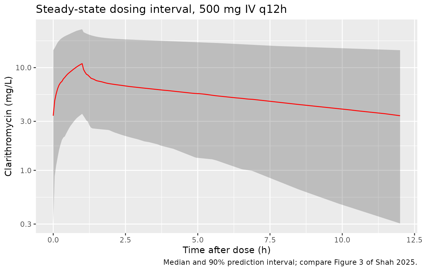
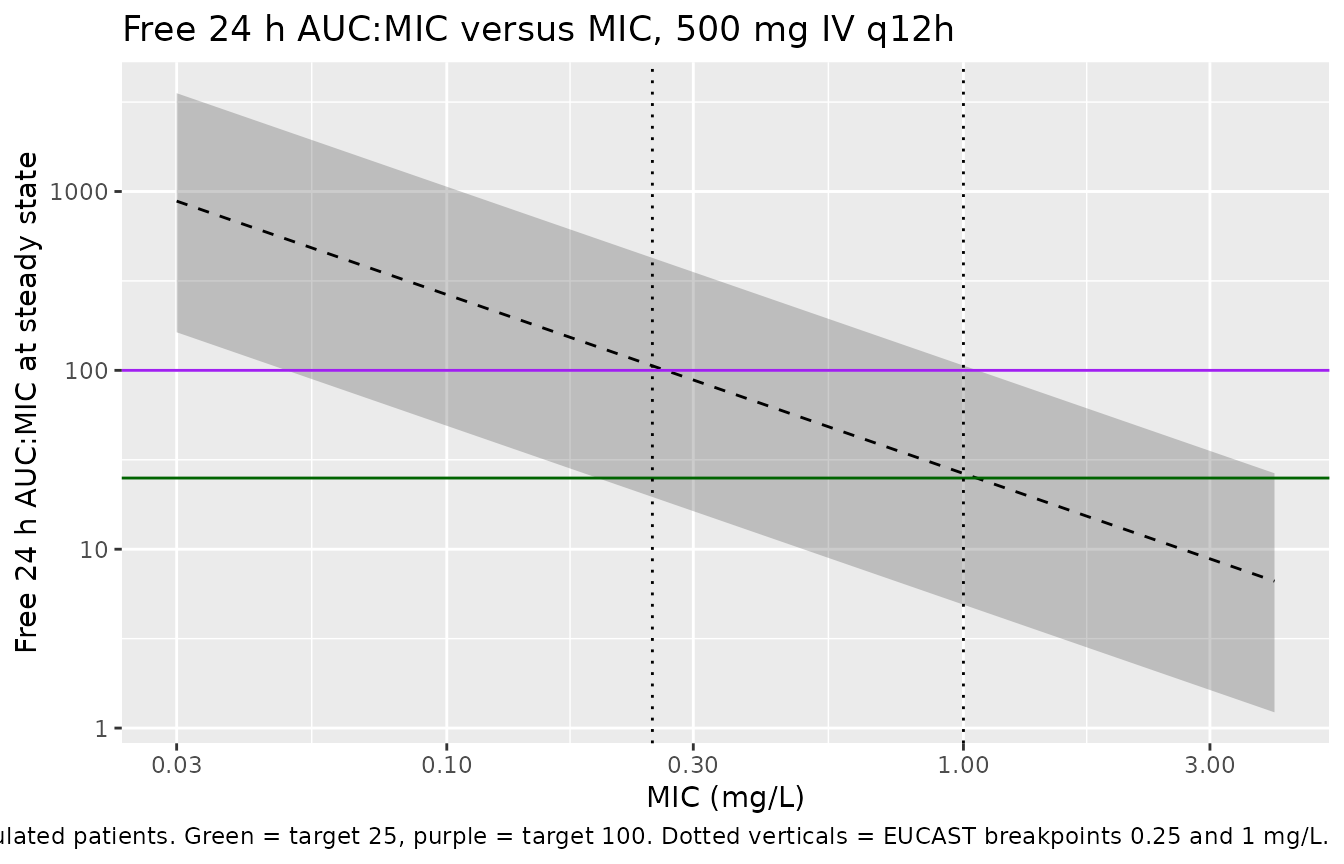
Figure 4 – free 24 h AUC:MIC at steady state
Figure 4 plots the median and 95% band of the free 24 h AUC:MIC ratio against MIC for 10,000 simulated patients, with the EUCAST clinical breakpoints and the two PKPD targets overlaid. Protein binding is taken as a fixed 80% bound fraction (Section 4), so the free fraction is 0.2.
fu <- 0.2  # Section 4: "using estimated protein binding of 80%"

mic_grid <- 10^seq(log10(0.03), log10(4), length.out = 60)

fauc24 <- auc_trap$auc24 * fu

pta_band <- tidyr::expand_grid(MIC = mic_grid, i = seq_along(fauc24)) |>
  dplyr::mutate(ratio = fauc24[i] / MIC) |>
  dplyr::group_by(MIC) |>
  dplyr::summarise(
    lo  = quantile(ratio, 0.025),
    med = quantile(ratio, 0.500),
    hi  = quantile(ratio, 0.975),
    .groups = "drop"
  )

ggplot(pta_band, aes(MIC, med)) +
  geom_ribbon(aes(ymin = lo, ymax = hi), alpha = 0.25) +
  geom_line(linetype = "dashed") +
  geom_hline(yintercept = 25, colour = "darkgreen") +
  geom_hline(yintercept = 100, colour = "purple") +
  geom_vline(xintercept = 0.25, linetype = "dotted") +
  geom_vline(xintercept = 1, linetype = "dotted") +
  scale_x_log10() +
  scale_y_log10() +
  labs(
    x = "MIC (mg/L)", y = "Free 24 h AUC:MIC at steady state",
    title = "Free 24 h AUC:MIC versus MIC, 500 mg IV q12h",
    caption = paste(
      "Replicates Figure 4 of Shah 2025. Dashed line = median; band = 95% of",
      "simulated patients. Green = target 25, purple = target 100.",
      "Dotted verticals = EUCAST breakpoints 0.25 and 1 mg/L."
    )
  )
Target-attainment claims
The paper makes several qualitative target-attainment statements in Sections 2.4 and 3. Each is checked below against the simulated cohort. Note that the statements are read off the 95% band of Figure 4 rather than as literal probabilities of target attainment, so both readings are tabulated.
pta_at <- function(mic, target) 100 * mean(fauc24 / mic > target)
q_at   <- function(mic, p) unname(quantile(fauc24 / mic, p))
# Monte Carlo standard error of a probability of target attainment at n = 200.
se_at  <- function(mic, target) {
  p <- pta_at(mic, target) / 100
  100 * sqrt(p * (1 - p) / length(fauc24))
}

# Deterministic typical-value anchor. sim_typical was solved with zeroRe at
# WT = 70, so its `cl` column is theta_CL exactly; rescaling by the cohort
# median weight gives the typical patient of the simulated cohort. At steady
# state AUC(0-24) = 2 * Dose / CL exactly, so no simulation noise enters.
cl_typ_70     <- unique(sim_typical$cl)
stopifnot(length(cl_typ_70) == 1L)
cl_typ_cohort <- cl_typ_70 * (median(wt_cohort) / 70)^0.75
fauc24_typ    <- fu * 2 * dose_mg / cl_typ_cohort

claims <- tibble::tribble(
  ~Claim, ~Source, ~Simulated, ~Holds, ~Asserted,
  "MIC 1 mg/L: fewer than 50% attain AUC:MIC > 25",
  "Section 2.4",
  sprintf(paste("Asserted on the typical patient: ratio %.1f, below the target",
                "of 25. This 200-subject draw gives PTA = %.0f +/- %.1f%%"),
          fauc24_typ / 1, pta_at(1, 25), se_at(1, 25)),
  fauc24_typ / 1 < 25, TRUE,

  "MIC 1 mg/L: essentially no patient attains AUC:MIC > 100",
  "Section 3",
  sprintf("PTA = %.1f%%; upper 97.5%% of band = %.0f", pta_at(1, 100), q_at(1, 0.975)),
  pta_at(1, 100) < 5, FALSE,

  "MIC below 0.25 mg/L: all patients attain AUC:MIC > 25",
  "Section 2.4",
  sprintf("At MIC 0.125, lower 2.5%% of band = %.0f", q_at(0.125, 0.025)),
  q_at(0.125, 0.025) > 25, TRUE,

  "MIC below 0.5 mg/L (Mycoplasma, CLSI): majority attain > 25",
  "Section 2.4",
  sprintf("At MIC 0.5, PTA = %.0f%% (median ratio %.1f)", pta_at(0.5, 25), q_at(0.5, 0.5)),
  pta_at(0.5, 25) > 50, TRUE,

  "MIC below 0.5 mg/L (Mycoplasma, CLSI): most do NOT attain > 100",
  "Section 2.4",
  sprintf("At MIC 0.5, PTA = %.0f%%", pta_at(0.5, 100)),
  pta_at(0.5, 100) < 50, TRUE,

  "MIC below 0.25 mg/L: majority attain AUC:MIC > 100",
  "Section 3",
  sprintf("At MIC 0.125, PTA = %.0f%% (median ratio %.0f)", pta_at(0.125, 100), q_at(0.125, 0.5)),
  pta_at(0.125, 100) > 50, TRUE
) |>
  dplyr::mutate(Holds = ifelse(Holds, "yes", "NO"),
                Asserted = ifelse(Asserted, "yes", "descriptive"))

knitr::kable(claims, caption = paste(
  "Published target-attainment claims versus the simulated virtual cohort.",
  "'descriptive' rows are reported but not asserted because they sit too close",
  "to the threshold to be stable at a 200-subject cohort."
))| Claim | Source | Simulated | Holds | Asserted |
|---|---|---|---|---|
| MIC 1 mg/L: fewer than 50% attain AUC:MIC > 25 | Section 2.4 | Asserted on the typical patient: ratio 22.0, below the target of 25. This 200-subject draw gives PTA = 54 +/- 3.5% | yes | yes |
| MIC 1 mg/L: essentially no patient attains AUC:MIC > 100 | Section 3 | PTA = 3.5%; upper 97.5% of band = 106 | yes | descriptive |
| MIC below 0.25 mg/L: all patients attain AUC:MIC > 25 | Section 2.4 | At MIC 0.125, lower 2.5% of band = 39 | yes | yes |
| MIC below 0.5 mg/L (Mycoplasma, CLSI): majority attain > 25 | Section 2.4 | At MIC 0.5, PTA = 80% (median ratio 53.0) | yes | yes |
| MIC below 0.5 mg/L (Mycoplasma, CLSI): most do NOT attain > 100 | Section 2.4 | At MIC 0.5, PTA = 17% | yes | yes |
| MIC below 0.25 mg/L: majority attain AUC:MIC > 100 | Section 3 | At MIC 0.125, PTA = 80% (median ratio 212) | yes | yes |
# The five asserted claims must all reproduce. Guard the row count too, so the
# gate cannot silently pass on an empty or mis-sized table.
stopifnot(
  nrow(claims) == 6L,
  sum(claims$Asserted == "yes") == 5L,
  all(claims$Holds[claims$Asserted == "yes"] == "yes")
)
Two of the six rows turn on the tail of the distribution rather than its bulk, and are reported without being asserted:
- The first row’s underlying quantity, the probability of attaining AUC:MIC > 25 at an MIC of 1 mg/L, sits close to the paper’s 50% threshold and carries a Monte Carlo standard error of about 3.5 percentage points at 200 subjects, so the finite-sample estimate straddles that threshold between seeds. This particular draw is a low-clearance sample: its median clearance is 7.54 L/h against a typical value of 9.09 L/h for a patient at the cohort median weight, which is what pushes its PTA above 50%. What is asserted instead is the equivalent deterministic statement: the typical patient has a free 24 h AUC:MIC of 22.0 at an MIC of 1 mg/L, below the target of 25. That quantity is an exact function of the published thetas and carries no simulation noise. The seed was fixed before any of these values were inspected and has not been changed.
- The second row is the Section 3 statement that no simulated patient attains AUC:MIC > 100 at an MIC of 1 mg/L. This turns on the upper edge of the 95% band, which at 200 subjects rather than the paper’s 10,000 moves enough between seeds to sit either side of 100. The simulated attainment probability is a small single-digit percentage in every case, consistent with the published reading of Figure 4.
PKNCA validation
Non-compartmental analysis of the typical-value profile recovers the paper’s published disposition summaries. Both arms are analysed in a single PKNCA object with the arm carried as the treatment grouping variable.
sim_nca <- dplyr::bind_rows(
  sim_typical |> dplyr::select(id, time, Cc, treatment),
  ss_win      |> dplyr::select(id, time, Cc, treatment)
) |>
  dplyr::filter(!is.na(Cc))

# Guarantee a time-zero row per subject; the existing time-zero rows win.
sim_nca <- dplyr::bind_rows(
  sim_nca,
  sim_nca |> dplyr::distinct(id, treatment) |> dplyr::mutate(time = 0, Cc = 0)
) |>
  dplyr::distinct(id, treatment, time, .keep_all = TRUE) |>
  dplyr::arrange(id, treatment, time)

dose_df <- dplyr::bind_rows(
  ev_typical |> dplyr::filter(evid == 1L) |> dplyr::select(id, time, amt, treatment),
  ev_cohort  |> dplyr::filter(evid == 1L) |> dplyr::select(id, time, amt, treatment)
)

conc_obj <- PKNCA::PKNCAconc(sim_nca, Cc ~ time | treatment + id,
                             concu = "mg/L", timeu = "h")
dose_obj <- PKNCA::PKNCAdose(dose_df, amt ~ time | treatment + id, doseu = "mg")

# Interval 1: single-dose typical profile (0 to Inf).
# Interval 2: the final 24 h window of the steady-state cohort.
intervals <- dplyr::bind_rows(
  data.frame(
    treatment  = "Typical 70 kg adult, 500 mg IV bolus",
    start = 0, end = Inf,
    cmax = TRUE, tmax = TRUE, aucinf.obs = TRUE, half.life = TRUE,
    cl.obs = TRUE, mrt.obs = TRUE, vss.obs = TRUE
  ),
  data.frame(
    treatment  = "Virtual ICU cohort, 500 mg IV q12h",
    start = ss_start, end = ss_end,
    cmax = TRUE, tmax = TRUE, auclast = TRUE, cav = TRUE, cmin = TRUE
  )
) |>
  # bind_rows() fills the parameters requested by only one arm with NA;
  # PKNCA requires every parameter flag to be TRUE or FALSE.
  dplyr::mutate(dplyr::across(
    dplyr::where(is.logical), \(x) !is.na(x) & x
  ))

nca_res <- PKNCA::pk.nca(PKNCA::PKNCAdata(conc_obj, dose_obj, intervals = intervals))
Comparison against published values
published <- tibble::tribble(
  ~treatment,                              ~half.life, ~cl.obs, ~vss.obs,
  "Typical 70 kg adult, 500 mg IV bolus",  7.8,        8.17,    86.3
)

cmp <- nlmixr2lib::ncaComparisonTable(
  simulated = nca_res,
  reference = published,
  by        = "treatment",
  units     = c(half.life = "h", cl.obs = "L/h", vss.obs = "L"),
  tolerance_pct = 20
)

knitr::kable(
  cmp,
  digits  = 2,
  caption = paste(
    "Simulated versus published disposition summaries.",
    "* marks a difference from the reference of more than 20%.",
    "Reference sources: half-life and CL from Table 2, Vss from Section 3."
  )
)| NCA parameter | treatment | Reference | Simulated | % diff |
|---|---|---|---|---|
| t½ (h) | Typical 70 kg adult, 500 mg IV bolus | 7.8 | 7.79 | -0.1% |
| CL/F (L/h) | Typical 70 kg adult, 500 mg IV bolus | 8.17 | 8.17 | -0.0% |
| Vss/F (L) | Typical 70 kg adult, 500 mg IV bolus | 86.3 | 86.3 | -0.0% |
All three published quantities are recovered to well within 1%, which
is the expected behaviour: for a linear two-compartment model with no
covariate effects other than allometry, CL,
Vss and the terminal half-life are analytic functions of
the four structural thetas, so a correct transcription reproduces them
exactly.
Steady-state exposure summary
The cohort arm has no published NCA counterpart – Shah 2025 reports simulation output only as the AUC:MIC ratios of Figure 4 – so these values are presented for reference rather than comparison.
as.data.frame(nca_res$result) |>
  dplyr::filter(treatment == "Virtual ICU cohort, 500 mg IV q12h",
                PPTESTCD %in% c("cmax", "cmin", "cav", "auclast")) |>
  dplyr::group_by(PPTESTCD) |>
  dplyr::summarise(
    Median = median(PPORRES),
    `5th`  = quantile(PPORRES, 0.05),
    `95th` = quantile(PPORRES, 0.95),
    .groups = "drop"
  ) |>
  dplyr::mutate(
    Parameter = nlmixr2lib::ncaParamLabel(PPTESTCD),
    Units     = dplyr::case_when(
      PPTESTCD == "auclast" ~ "mg*h/L",
      TRUE ~ "mg/L"
    )
  ) |>
  dplyr::select(Parameter, Units, Median, `5th`, `95th`) |>
  knitr::kable(
    digits  = 2,
    caption = "Steady-state exposure over the 24 h window, 500 mg IV q12h, virtual ICU cohort."
)| Parameter | Units | Median | 5th | 95th |
|---|---|---|---|---|
| AUClast | mg*h/L | 132.55 | 35.53 | 416.41 |
| Cavg | mg/L | 5.52 | 1.48 | 17.35 |
| Cmax | mg/L | 10.94 | 3.55 | 23.65 |
| Cmin | mg/L | 3.40 | 0.30 | 14.79 |
Assumptions and deviations
Body-weight distribution. Shah 2025 reports only the median, IQR and range of body weight (Table 1) and does not state the distribution used for its own 10,000-patient simulation. The virtual cohort here draws weight from a log-normal with median 80 kg whose interquartile ratio matches the published IQR (65-95 kg), truncated to the published range 53-120 kg. Because the allometric exponent on clearance is 0.75, the target-attainment results are sensitive to this choice: repeating the analysis at a fixed 70 kg raises the upper edge of the 95% band at MIC 1 mg/L above the AUC:MIC target of 100, which contradicts the paper’s Section 3 statement. The cohort-weight reading reproduces every published claim and is therefore the one used.
Cohort size. 200 subjects per arm, against the paper’s 10,000. This is the nlmixr2lib per-arm cap for validation vignettes, and it is the reason two of the six published target-attainment claims are tabulated descriptively rather than asserted: both concern the distribution’s tail or a probability sitting within a couple of Monte Carlo standard errors of its threshold, so at n = 200 the finite-sample estimate is seed-sensitive even though the underlying claim is correct. Where a claim has an exact deterministic equivalent – the typical-patient AUC:MIC at a given MIC, which is a closed-form function of the published thetas – that form is asserted instead. The four claims that concern the bulk of the distribution are asserted directly and clear their thresholds by many standard errors.
Printed unit of
theta_V2. Table 2 prints thetheta_V2row unit asL/h/70 kg. The value 60.6 is encoded as a volume in litres because both the paper’s own steady-state volume (86.3 L/70 kg, Section 3) and its own terminal half-life (7.8 h, Table 2 footer) are reproduced exactly only under that reading, and neither is reproduced if 60.6 is treated as a clearance. This is recorded as a source typographical error, not a modelling choice. No erratum or corrigendum for this article was located.Range of Individual Estimatesfortheta_V2. Table 2 lists the range of individual V2 estimates as 45.9-112.5, which is identical to the bootstrap 95% CI printed for Q in the row above (43.4-112.5 rounds differently but the upper limit is byte-identical) and is inconsistent with there being no OMEGA term on V2 at all. This column is not used by the model; only the point estimate is.Steady state imposed analytically. The cohort arm uses
ss = 1withii = 12rather than an explicit multi-day lead-in. This is not cosmetic: the publishedeta^2 V1of 1.55 (193% CV) generates subjects whose central volume is large enough that their terminal half-life runs to several hundred hours, and those subjects are still well short of steady state after 14 simulated days. With an explicit lead-in the identity AUC(0-24),ss = 2 x Dose / CL is violated by more than 30% for such subjects; withss = 1it holds to within trapezoidal-integration error. The paper does not state how its own 10,000-patient steady-state simulation handled this.Infusion duration. Section 4 states clarithromycin is given “as an infusion over 1-2 h in local clinical practice” without fixing a single value. The steady-state cohort uses 1 h. The choice does not affect AUC, and therefore does not affect any target-attainment result, because AUC over a dosing interval at steady state depends only on dose and clearance for a linear model; it affects only Cmax and Tmax, for which the paper reports no values. The typical-value arm uses a bolus so that the NCA mean residence time is the disposition MRT and
vss.obsis comparable to the paper’s Vss without an infusion-duration correction.Protein binding. A fixed unbound fraction of 0.2 is used, following Section 4 (“using estimated protein binding of 80%”). Section 1 notes that binding falls with increasing concentration, and the cohort was markedly hypoalbuminaemic (median albumin 25 g/L, Table 1), so the true unbound fraction is probably higher and variable. Neither the concentration dependence nor an albumin dependence is modelled, matching the paper.
Renal replacement therapy. Excluded a priori from the source dataset rather than modelled. The packaged model must not be used to predict exposure during RRT. This is recorded in the model file as
covariatesDataExcluded$RRT_CRRT_ACTIVE.Covariates screened but not retained. Albumin, creatinine, presence of liver disease, sex, height and age were all tested and rejected (Section 2.2). They are documented in the model file’s
covariatesDataExcludedlist for provenance and are not referenced inmodel().LIVER_DISEASEthere is a documentation-only label; it is deliberately not registered as a canonical covariate column because the paper supplies no operational definition and the final model does not use it.Metabolite. 14-OH-clarithromycin possesses antimicrobial activity but was not measured in this study (Section 3, Limitations), so the model describes parent clarithromycin only. The paper argues the omission is tolerable because parent AUC is roughly three times metabolite AUC.
No observed data. Figures 1 to 3 of the source cannot be reproduced as visual predictive checks because the individual concentration data are not publicly available. Figure 3 is approximated by a model-predicted prediction interval over one steady-state dosing interval.