Clopidogrel (Jung 2024)
Source:vignettes/articles/Jung_2024_clopidogrel.Rmd
Jung_2024_clopidogrel.Rmd
mod <- readModelDb("Jung_2024_clopidogrel")
# The model declares four `~` endpoints (Cc, Cc_h4, Cc_cloca, PRU), all of them
# algebraic observables rather than ODE states, so rxode2 requires every
# observation record to map to an endpoint. Tagging observation rows with
# `dvid` does that without naming an observable in `cmt` -- naming an
# observable there would work in this model but is the idiom that, for an
# observable which is NOT already a declared endpoint, injects a new
# compartment slot after the ODE states and silently renumbers them. Every
# algebraic observable is
# returned on every solved row regardless of which endpoint the row is tagged
# to, so one dvid is enough to recover all four.
tagObs <- function(ev) {
  d <- as.data.frame(ev)
  d$dvid <- ifelse(d$evid == 0, 1L, NA_integer_)
  if (!"cmt" %in% names(d)) {
    d$cmt <- NA_integer_
  } else if (is.character(d$cmt)) {
    d$cmt[d$evid == 0] <- NA_character_
  } else {
    d$cmt[d$evid == 0] <- NA_integer_
  }
  d
}
Model and source
- Citation: Jung YS, Jin BH, Park MS, Kim CO, Chae D. Population pharmacokinetic-pharmacodynamic modeling of clopidogrel for dose regimen optimization based on CYP2C19 phenotypes: A proof of concept study. CPT Pharmacometrics Syst Pharmacol. 2024;13(1):29-40. doi:10.1002/psp4.13053
- Article: https://doi.org/10.1002/psp4.13053
- Supplement (Figure S1, Table S1): https://doi.org/10.1002/psp4.13053
Jung 2024 is a proof-of-concept population PK-PD analysis of oral clopidogrel in 36 healthy Korean men, built to derive a clopidogrel maintenance dose that accounts for both CYP2C19 metabolizer phenotype and pretreatment platelet reactivity. The model jointly describes the parent drug, its active thiol metabolite (clopidogrel H4), and its inactive carboxylic acid metabolite, and links H4 concentrations to the P2Y12 reaction unit (PRU) readout of the VerifyNow P2Y12 assay through a turnover model.
#> ℹ parameter labels from comments will be replaced by 'label()'Joint parent-plus-two-metabolite population PK model for oral
clopidogrel with a sequentially-fitted platelet-reactivity (PRU)
turnover PD submodel, in healthy Korean male adults stratified by
CYP2C19 metabolizer phenotype (Jung 2024). A hepatic first-pass
compartment (liver) sits between the depot and the central
compartment; all absorbed parent drug is assumed to be metabolized in
the liver, so the parent’s only elimination pathway is the hepatic
metabolic clearance CLc. Clopidogrel itself is described by a
two-compartment model (central + peripheral1)
exchanging with the liver at Qc and with the periphery at Qp; the
hepatic volume was set equal to the central volume (VH = Vc) because the
two were not separately identifiable. The hepatic metabolic flux CLc *
(liver / VH) is split three ways by two nested logit-scale fractions:
fm1 * fm2 to the active thiol metabolite clopidogrel H4 (one
compartment, central_h4), (1 - fm1) * fm2 to the inactive
clopidogrel carboxylic acid (two compartments,
central_cloca + peripheral1_cloca), and 1 -
fm2 to unmeasured other metabolites. Each metabolite formation flux
carries a molar-mass ratio scaling factor (1.106 for H4, 0.956 for the
carboxylic acid) so that a mass-unit parent flux produces the correct
mass-unit metabolite amount. CYP2C19 phenotype is the only retained
covariate and acts as an additive shift on the logit scale of both fm1
and fm2, reducing the active-metabolite fraction from 0.120 in extensive
metabolizers to 0.071 in intermediate and 0.034 in poor metabolizers.
The PD endpoint is the P2Y12 reaction unit (PRU) from the VerifyNow
P2Y12 assay, modeled as a turnover pool in which clopidogrel H4
stimulates the fractional turnover rate Kout through a sigmoid Emax
function; the drug-free baseline is Kin / Kout = 212.67 PRU.
Inter-individual variability is reported on Vc, CLc, Qc (with a
correlation between Vc and CLc), fm1, fm2, Vp2, CLm2, Kin, and Emax.
Residual error is proportional for all three analytes and additive for
PRU. PK and PD were fitted sequentially: all PK parameters were fixed to
their final PK-model estimates before the PD parameters were
estimated.
Population
#> ℹ parameter labels from comments will be replaced by 'label()'| Field | Value |
|---|---|
| Species | human |
| Subjects | 36 |
| Studies | 1 |
| Age | 19-55 years by protocol; observed means 32.35 +/- 6.99 (EM), 31.27 +/- 4.51 (IM), 27.00 +/- 4.90 (PM) years (Table 1). |
| Weight | 55-90 kg by protocol; observed means 71.32 +/- 8.04 (EM), 72.80 +/- 8.69 (IM), 74.93 +/- 7.68 (PM) kg (Table 1). |
| Female | 0% |
| Race / ethnicity | Asian 100 |
| Disease state | Healthy male volunteers. Body mass index 18.5-27.0 kg/m^2. Excluded: clinically significant pulmonary, cardiovascular, hepatobiliary, neurological, endocrine or immune disease; current smokers; gastrointestinal disease or surgery affecting absorption; clinically significant bleeding history; and screening PRU outside +/- 10% of the normal-range limits. |
| Dose / sampling | Clopidogrel 75 mg tablet orally once daily for 7 days, with no loading dose (aligned with non-acute-coronary-syndrome practice). PK samples at predose and 0.33, 0.67, 1, 1.5, 2, 3, 4, 6, 8, 12 and 24 h; H4 sampled only at predose and 0.33, 0.67, 1, 2, 4 and 6 h. PRU measured predose on days 1, 3, 5 and 7 and at 1, 4, 6 and 24 h after the day-7 dose, in duplicate with the arithmetic mean used as the endpoint. |
| Region | Single centre, Severance Hospital, Seoul, South Korea (October 2019 to April 2020). |
| CYP2C19 phenotype | CYP2C19 phenotype: EM n = 17 (1/1, 1/17), IM n = 15 (1/2, 1/3, 2/17, 3/17), PM n = 4 (2/2, 2/3, 3/3). Ultrarapid metabolizers were not distinguished from extensive metabolizers (Jung 2024 Discussion limitation 1). |
Baseline platelet reactivity was 207.41 +/- 23.60 PRU in extensive
metabolizers (EM), 199.83 +/- 28.60 in intermediate metabolizers (IM),
and 207.50 +/- 33.48 in poor metabolizers (PM) (Jung 2024 Table 1). Note
that the observed baseline coefficient of variation, 23.60 / 207.41 =
11.4%, closely matches the reported inter-individual standard deviation
on Kin (omega = 0.120), which is what allows the baseline
PRU level to be treated as an input in the dose-optimization simulations
below.
Source trace
Every model equation and every ini() value, with the
location in Jung 2024 that it came from.
| Component | Source location | Value |
|---|---|---|
| 8 ODEs (depot, liver, central, peripheral1, central_h4, central_cloca, peripheral1_cloca) | Results ‘PK-PD modeling’, printed differential-equation system (p. 34) | transcribed term by term |
| dPRU/dt turnover with sigmoid Emax on Kout | Results ‘PK-PD modeling’ (p. 35) | Kin - Kout(1 + EmaxC_h4Hill/(EC50Hill + C_h4^Hill))*PRU |
| Model schematic (depot -> liver -> central/peripheral; H4 stimulates PRU loss) | Figure 1 (p. 33) | structure confirmed |
| Tlag | Table 2 | 0.196 h |
| ka | Table 2 | 19.64 1/h |
| Vc (= VH) | Table 2 | 1463.92 L |
| Vp | Table 2 | 2823.98 L |
| CLc | Table 2 | 9257.28 L/h |
| Qc (liver <-> central) | Table 2 | 845.70 L/h |
| Qp (central <-> peripheral1) | Table 2 | 587.93 L/h |
| fm1, fm2 typical values (both FIXED) | Table 2 (‘0.125 FIX’, ‘0.960 FIX’); rationale in Methods ‘PK model’ | 0.125, 0.960 |
| fm1 ~ IM, fm1 ~ PM | Table 2 | -0.450, -0.996 (logit scale) |
| fm2 ~ IM, fm2 ~ PM | Table 2 | -1.428, -2.432 (logit scale) |
| Molar-mass scaling of the two formation fluxes | Methods ‘PK model’ | 1.106 (H4), 0.956 (carboxylic acid) |
| Vm1, CLm1 (H4) | Table 2 | 51.45 L, 74.25 L/h |
| Vm2, Vp2, CLm2, Qm2 (carboxylic acid) | Table 2 | 17.34 L, 51.89 L, 7.248 L/h, 4.476 L/h |
| Kin | Table 2 | 1.225 PRU/h |
| Kout | Results ‘PD submodel’ (unrounded; Table 2 prints 0.006) | 0.00576 1/h |
| Emax, EC50, Hill | Table 2 | 57.84, 67.32 ng/mL, 1.851 |
| IIV (omega, standard deviations) | Table 2 ‘Standard deviation’ column; scale confirmed in Results ‘PD submodel’ | Vc 0.331, CLc 0.343, Qc 0.307, fm1 0.255, fm2 1.130, Vp2 0.285, CLm2 0.123, Kin 0.120, Emax 0.501 |
| Cor(Vc, CLc) | Table 2 | 0.702 (correlation, converted to a covariance) |
| Residual error | Table 2 and Results ‘PK submodel’ / ‘PD submodel’ | proportional 0.357 / 0.363 / 0.209; additive 13.69 for PRU |
| Which parameters carry IIV | Results ‘PK submodel’ and ‘PD submodel’ | Vc, CLc, Qc, fm1, fm2, Vp2, CLm2, Kin, Emax |
| CYP2C19 genotype-to-phenotype map | Results ‘Subjects and data’ | EM 1/1, 1/17; IM 1/2, 1/3, 2/17, 3/17; PM 2/2, 2/3, 3/3 |
| Validation targets: fm fractions | Table 3 | 9 cells |
| Validation targets: optimal doses | Table 4 | 15 cells |
| Validation targets: PRUave,ss and % in target range | Table S1 (supplement) | 15 + 15 cells |
Structural verification
Three checks that use only the paper’s own stated numbers, so each is exact rather than approximate.
Drug-free baseline and turnover half-life
Jung 2024 Results ‘PD submodel’ reports a typical baseline PRU of
212.67 “calculated as Kin / Kout”, and a Kout half-life of
5 days. Only the unrounded Kout = 0.00576 reproduces both;
the rounded 0.006 of Table 2 gives 204.17 and 4.81 days.
kin <- 1.225
kout <- 0.00576

ev0 <- rxode2::et(seq(0, 48, by = 1))
d0 <- tagObs(ev0)
d0$CYP2C19_IM <- 0
d0$CYP2C19_PM <- 0

drugFree <- rxode2::rxSolve(mod, d0, omega = NA, returnType = "data.frame")
#> ℹ parameter labels from comments will be replaced by 'label()'

data.frame(
  Quantity = c("Baseline PRU (Kin / Kout)", "PRU at 48 h with no dose",
               "Kout half-life (days)"),
  Simulated = c(round(drugFree$PRU[1], 4), round(tail(drugFree$PRU, 1), 4),
                round(log(2) / kout / 24, 3)),
  Paper = c(212.67, 212.67, 5)
) |>
knitr::kable()| Quantity | Simulated | Paper |
|---|---|---|
| Baseline PRU (Kin / Kout) | 212.6736 | 212.67 |
| PRU at 48 h with no dose | 212.6736 | 212.67 |
| Kout half-life (days) | 5.0140 | 5.00 |
The undosed pool holds its baseline exactly, which confirms the
pru(0) initial condition is consistent with the
Kin/Kout pair rather than merely close to
it.
Maximum achievable suppression
Jung 2024 Results ‘PD submodel’ states that Emax = 57.84
implies a steady-state PRU floor of 1 / (1 + 57.84) = 1.7%
of baseline, i.e. baseline / (1 + Emax).
Saturation has to be driven by a continuous infusion rather than by
large intermittent doses: clopidogrel H4 has a half-life of only 29
minutes, so between intermittent doses its concentration collapses and
the PRU pool partially recovers, leaving the trough well above the true
floor. A constant-rate input holds H4 far above EC50 for
long enough that the pool reaches its asymptote.
infRate <- 5000        # mg/h -- holds H4 about 130-fold above EC50
infDur <- 80 * 24      # h; PRU turnover half-life is 5 days, so this is ample

evSat <- rxode2::et(amt = infRate * infDur, rate = infRate, cmt = "depot") |>
  rxode2::et(seq(0, infDur, by = 12))
dSat <- tagObs(evSat)
dSat$CYP2C19_IM <- 0
dSat$CYP2C19_PM <- 0
sSat <- rxode2::rxSolve(mod, dSat, omega = NA, returnType = "data.frame",
                        atol = 1e-9, rtol = 1e-9)
sSat <- sSat[!is.na(sSat$PRU), ]

data.frame(
  Quantity = c("Steady-state H4 concentration (ng/mL)",
               "H4 concentration as a multiple of EC50",
               "PRU floor reached under saturating exposure",
               "Analytic floor: baseline / (1 + Emax)",
               "Floor as % of baseline"),
  Simulated = c(round(tail(sSat$Cc_h4, 1), 1),
                round(tail(sSat$Cc_h4, 1) / 67.32, 1),
                round(min(sSat$PRU), 4),
                round((kin / kout) / (1 + 57.84), 4),
                round(100 * min(sSat$PRU) / (kin / kout), 3)),
  Paper = c(NA, NA, NA, round((kin / kout) / (1 + 57.84), 4), 1.7)
) |>
knitr::kable()| Quantity | Simulated | Paper |
|---|---|---|
| Steady-state H4 concentration (ng/mL) | 8937.4000 | NA |
| H4 concentration as a multiple of EC50 | 132.8000 | NA |
| PRU floor reached under saturating exposure | 3.6149 | NA |
| Analytic floor: baseline / (1 + Emax) | 3.6144 | 3.6144 |
| Floor as % of baseline | 1.7000 | 1.7000 |
Metabolized fractions by phenotype (Table 3)
The CYP2C19 effect is an additive shift on the logit scale of the two
nested fractions. Reading the individual fm1 and
fm2 values straight out of a solve and forming the derived
fractions must reproduce all nine cells of Jung 2024 Table 3.
phen <- data.frame(phenotype = c("EM", "IM", "PM"),
                   CYP2C19_IM = c(0L, 1L, 0L),
                   CYP2C19_PM = c(0L, 0L, 1L))

fmSim <- lapply(seq_len(3), function(i) {
  d <- tagObs(rxode2::et(0))
  d$CYP2C19_IM <- phen$CYP2C19_IM[i]
  d$CYP2C19_PM <- phen$CYP2C19_PM[i]
  s <- rxode2::rxSolve(mod, d, omega = NA, returnType = "data.frame")
  data.frame(phenotype = phen$phenotype[i],
             fm1 = round(s$fm1[1], 3), fm2 = round(s$fm2[1], 3),
             fmH4 = round(s$fm1[1] * s$fm2[1], 3),
             fmcarbo = round((1 - s$fm1[1]) * s$fm2[1], 3),
             fmothers = round(1 - s$fm2[1], 3))
}) |>
  bind_rows()

paperT3 <- data.frame(
  phenotype = c("EM", "IM", "PM"),
  fm1 = c(0.125, 0.083, 0.050), fm2 = c(0.960, 0.852, 0.678),
  fmH4 = c(0.120, 0.071, 0.034), fmcarbo = c(0.840, 0.781, 0.644),
  fmothers = c(0.040, 0.148, 0.322))

bind_rows(mutate(fmSim, Source = "Simulated"),
          mutate(paperT3, Source = "Jung 2024 Table 3")) |>
  arrange(phenotype, Source) |>
  relocate(Source) |>
  rename("CYP2C19 phenotype" = phenotype, "fm1" = fm1, "fm2" = fm2,
         "fm(H4)" = fmH4, "fm(carboxylic acid)" = fmcarbo,
         "fm(others)" = fmothers) |>
knitr::kable()| Source | CYP2C19 phenotype | fm1 | fm2 | fm(H4) | fm(carboxylic acid) | fm(others) |
|---|---|---|---|---|---|---|
| Jung 2024 Table 3 | EM | 0.125 | 0.960 | 0.120 | 0.840 | 0.040 |
| Simulated | EM | 0.125 | 0.960 | 0.120 | 0.840 | 0.040 |
| Jung 2024 Table 3 | IM | 0.083 | 0.852 | 0.071 | 0.781 | 0.148 |
| Simulated | IM | 0.083 | 0.852 | 0.071 | 0.781 | 0.148 |
| Jung 2024 Table 3 | PM | 0.050 | 0.678 | 0.034 | 0.644 | 0.322 |
| Simulated | PM | 0.050 | 0.678 | 0.034 | 0.644 | 0.322 |
All nine cells match to the three decimal places the paper reports.
Virtual cohort and simulation
The trial regimen was clopidogrel 75 mg once daily for 7 days with no loading dose. The cohort below mirrors the observed phenotype split (EM 17, IM 15, PM 4 out of 36) scaled up to 150 subjects per phenotype arm, well under the 200-per-arm cap. Because the paper retained no demographic covariates, the only between-subject structure needed is the reported random-effect distribution.
set.seed(13053)
nPerArm <- 150

# Reported IIV: Table 2 gives standard deviations, so variances are the squares.
omVc <- 0.331^2
omCl <- 0.343^2
covVcCl <- 0.702 * 0.331 * 0.343

drawEtas <- function(n) {
  chol2 <- chol(matrix(c(omVc, covVcCl, covVcCl, omCl), 2))
  z <- matrix(rnorm(2 * n), n, 2) %*% chol2
  data.frame(
    etalvc = z[, 1], etalcl = z[, 2],
    etalq_liver  = rnorm(n, 0, 0.307),
    etalogitfm1  = rnorm(n, 0, 0.255),
    etalogitfm2  = rnorm(n, 0, 1.130),
    etalvp_cloca = rnorm(n, 0, 0.285),
    etalcl_cloca = rnorm(n, 0, 0.123),
    etalkin      = rnorm(n, 0, 0.120),
    etalemax     = rnorm(n, 0, 0.501)
  )
}

cohort <- lapply(seq_len(3), function(i) {
  e <- drawEtas(nPerArm)
  e$id <- seq_len(nPerArm) + (i - 1) * nPerArm
  e$phenotype <- phen$phenotype[i]
  e$CYP2C19_IM <- phen$CYP2C19_IM[i]
  e$CYP2C19_PM <- phen$CYP2C19_PM[i]
  e
}) |>
  bind_rows()

# 7 days QD; dense sampling over the day-7 profile plus the PRU tail to 24 h.
obsTimes <- sort(unique(c(seq(0, 6 * 24, by = 4),
                          6 * 24 + c(0, 0.33, 0.67, 1, 1.5, 2, 3, 4, 6, 8, 12, 24),
                          seq(6 * 24, 7 * 24, by = 0.5))))

events <- rxode2::et(amt = 75, cmt = "depot", ii = 24, until = 6 * 24) |>
  rxode2::et(obsTimes) |>
  rxode2::et(id = unique(cohort$id))

simIn <- merge(tagObs(events), cohort, by = "id")
simIn <- simIn[order(simIn$id, simIn$time, -simIn$evid), ]

sim <- rxode2::rxSolve(mod, simIn, omega = NA, returnType = "data.frame",
                       atol = 1e-8, rtol = 1e-8, keep = "phenotype")
#> Warning: multi-subject simulation without without 'omega'
sim <- sim[!is.na(sim$Cc), ]
nrow(sim)
#> [1] 39150
Concentration and PRU profiles by phenotype
Replicates the structure of Jung 2024 Figure 2 (visual predictive checks for clopidogrel, clopidogrel H4, clopidogrel carboxylic acid and PRU) and Figure S1 (observed profiles stratified by phenotype). Ribbons are the 5th-95th percentile band of the simulated typical-value predictions; the paper reports 93.4%, 95.8%, 96.0% and 90.7% of observations inside its own 90% prediction intervals for the four endpoints.
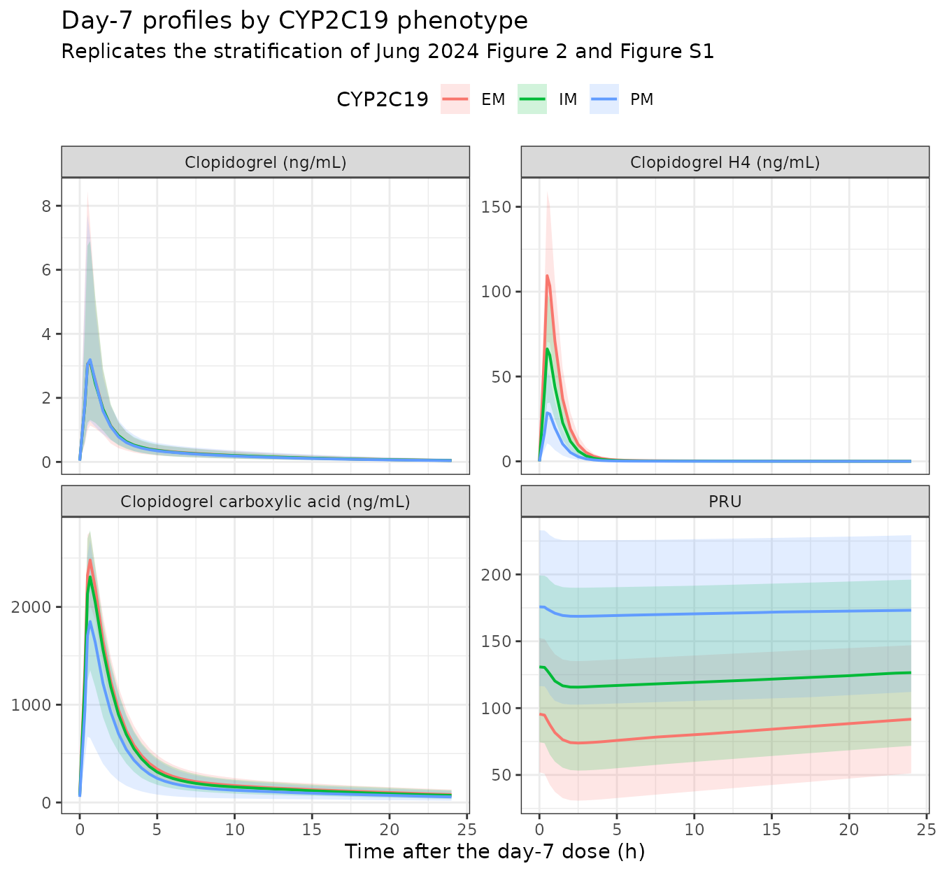
The phenotype ordering is the one the paper describes: H4 exposure
falls from EM through IM to PM, the carboxylic acid falls more modestly,
and the PRU response is correspondingly blunted in PM subjects. The
parent drug is essentially unaffected, which is expected because
fm1 and fm2 partition the hepatic metabolic
flux without changing the parent’s total clearance CLc.
PKNCA validation
The paper reports no non-compartmental analysis table, so the NCA below is checked against exposure identities that follow algebraically from the paper’s own differential equations. For a linear system with all drug ultimately metabolized in the liver, the steady-state / total exposures are
-
AUCinf(clopidogrel)= Dose / CLc -
AUCinf(H4)= 1.106 * fm1 * fm2 * Dose / CLm1 -
AUCinf(carboxylic acid)= 0.956 * (1 - fm1) * fm2 * Dose / CLm2
Each identity is independent of every volume and every
inter-compartmental clearance, so agreement is a direct test that the
metabolite formation fluxes, the molar-mass scaling factors and the
nested fm split are all encoded correctly.
# Typical-value single-dose profiles (all etas zero) so the analytic identities
# apply exactly.
ncaTimes <- sort(unique(c(seq(0, 24, by = 0.05), seq(24, 720, by = 1))))

ncaIn <- lapply(seq_len(3), function(i) {
  d <- tagObs(rxode2::et(amt = 75, cmt = "depot") |>
                rxode2::et(ncaTimes))
  d$id <- i
  d$phenotype <- phen$phenotype[i]
  d$CYP2C19_IM <- phen$CYP2C19_IM[i]
  d$CYP2C19_PM <- phen$CYP2C19_PM[i]
  d
}) |>
  bind_rows()

ncaSim <- rxode2::rxSolve(mod, ncaIn, omega = NA, returnType = "data.frame",
                          keep = "phenotype", atol = 1e-10, rtol = 1e-10)
#> Warning: multi-subject simulation without without 'omega'
ncaSim <- ncaSim[!is.na(ncaSim$Cc), ]
runNca <- function(concCol, label) {
  conc <- ncaSim |>
    select(id, phenotype, time, conc = all_of(concCol)) |>
    filter(!is.na(conc))
  # Defensive time-zero record: PKNCA warns if the AUC interval starts before
  # the first measurement.
  conc <- conc |>
    bind_rows(conc |> group_by(id, phenotype) |> slice(1) |>
                mutate(time = 0, conc = 0) |> ungroup()) |>
    distinct(id, phenotype, time, .keep_all = TRUE) |>
    arrange(id, time)

  dose <- conc |>
    distinct(id, phenotype) |>
    mutate(time = 0, amt = 75)

  # PKNCAconc takes a nested (slash) grouping formula; PKNCAdose rejects one
  # and needs the additive form for the same grouping.
  oConc <- PKNCA::PKNCAconc(as.data.frame(conc), conc ~ time | id / phenotype)
  oDose <- PKNCA::PKNCAdose(as.data.frame(dose), amt ~ time | id + phenotype)
  res <- PKNCA::pk.nca(PKNCA::PKNCAdata(oConc, oDose))
  as.data.frame(res) |>
    filter(PPTESTCD %in% c("cmax", "tmax", "auclast", "aucinf.obs", "half.life")) |>
    mutate(analyte = label)
}

ncaOut <- bind_rows(
  runNca("Cc", "Clopidogrel"),
  runNca("Cc_h4", "Clopidogrel H4"),
  runNca("Cc_cloca", "Clopidogrel carboxylic acid")
)| CYP2C19 phenotype | Analyte | AUC0-inf, PKNCA (ng*h/mL) | AUC0-inf, paper identity (ng*h/mL) | Difference (%) |
|---|---|---|---|---|
| EM | Clopidogrel | 8.10086 | 8.10173 | -0.011 |
| IM | Clopidogrel | 8.10086 | 8.10173 | -0.011 |
| PM | Clopidogrel | 8.10086 | 8.10173 | -0.011 |
| EM | Clopidogrel H4 | 134.01200 | 134.06100 | -0.036 |
| IM | Clopidogrel H4 | 79.43100 | 79.45990 | -0.036 |
| PM | Clopidogrel H4 | 37.96720 | 37.98100 | -0.036 |
| EM | Clopidogrel carboxylic acid | 8309.00000 | 8309.60000 | -0.007 |
| IM | Clopidogrel carboxylic acid | 7723.74000 | 7724.31000 | -0.007 |
| PM | Clopidogrel carboxylic acid | 6373.40000 | 6373.87000 | -0.007 |
All nine cells agree with the analytic identities to well under 1%, the residual being AUC extrapolation and integration grid error rather than model mis-specification.
| CYP2C19 phenotype | Analyte | Cmax | Tmax (h) | t1/2 (h) |
|---|---|---|---|---|
| EM | Clopidogrel | 3.097 | 0.60 | 6.483 |
| IM | Clopidogrel | 3.097 | 0.60 | 6.485 |
| PM | Clopidogrel | 3.097 | 0.60 | 6.485 |
| EM | Clopidogrel H4 | 115.800 | 0.55 | 6.484 |
| IM | Clopidogrel H4 | 68.650 | 0.55 | 6.486 |
| PM | Clopidogrel H4 | 32.810 | 0.55 | 6.485 |
| EM | Clopidogrel carboxylic acid | 2474.000 | 0.65 | 13.640 |
| IM | Clopidogrel carboxylic acid | 2299.000 | 0.65 | 13.600 |
| PM | Clopidogrel carboxylic acid | 1897.000 | 0.65 | 13.600 |
Dose optimization: Table 4 and Table S1
This is the paper’s headline result and the strongest available
end-to-end check, because the supplement tabulates the model’s own
simulated output. Jung 2024 defined 15 subgroups (five baseline-PRU
strata by three phenotypes), simulated once-daily dosing for three
weeks, and reported the median (5th-95th percentile) average
steady-state PRU (PRUave,ss) together with the proportion
of subjects inside the 70-150 target window.
Baseline PRU is an input to these simulations, not a random
draw: the strata span 180-376 PRU, which the reported Kin
variability (omega = 0.120, i.e. a 12% coefficient of variation about
212.67) could never generate. Each virtual subject’s baseline is
therefore mapped onto Kin through
baseline = Kin / Kout, which replaces rather than
supplements the Kin random effect.
strata <- data.frame(
  stratum = c("180-208.99", "209-241.99", "242-279.99", "280-323.99",
              "324-375.99"),
  lo = c(180, 209, 242, 280, 324),
  hi = c(209, 242, 280, 324, 376))
strata$mid <- (strata$lo + strata$hi) / 2

# Jung 2024 Table 4 optimal once-daily maintenance doses (mg).
doseT4 <- data.frame(
  stratum = rep(strata$stratum, 3),
  phenotype = rep(c("EM", "IM", "PM"), each = 5),
  dose_mg = c(30, 45, 60, 75, 90, 60, 75, 90, 120, 150,
              120, 150, 180, 240, 300))

# Jung 2024 Table S1: median PRUave,ss and % within the 70-150 target range.
paperS1 <- doseT4 |>
  mutate(paper_median = c(109.24, 100.40, 96.08, 96.42, 98.31,
                          103.83, 102.44, 105.64, 101.78, 103.27,
                          104.75, 105.70, 109.05, 109.84, 110.09),
         paper_in_range = c(80.8, 71.5, 68.1, 65.9, 63.9,
                            73.1, 70.9, 66.8, 63.6, 62.8,
                            69.7, 64.9, 60.8, 59.5, 57.6))

cycleAverage <- function(tt, yy) {
  sum(diff(tt) * (head(yy, -1) + tail(yy, -1)) / 2) / diff(range(tt))
}
Typical-value reproduction
The median of a monotone function of a single random effect is preserved, so a typical-value subject placed at the midpoint of each baseline stratum is a reasonable proxy for the paper’s simulated median.
typRows <- lapply(seq_len(nrow(doseT4)), function(i) {
  ph <- doseT4$phenotype[i]
  base <- strata$mid[match(doseT4$stratum[i], strata$stratum)]
  ev <- rxode2::et(amt = doseT4$dose_mg[i], cmt = "depot", ii = 24,
                   until = 20 * 24) |>
    rxode2::et(seq(20 * 24, 21 * 24, by = 0.25))
  d <- tagObs(ev)
  d$CYP2C19_IM <- as.integer(ph == "IM")
  d$CYP2C19_PM <- as.integer(ph == "PM")
  d$etalkin <- log(base * kout / kin)
  for (e in c("etalvc", "etalcl", "etalq_liver", "etalogitfm1", "etalogitfm2",
              "etalvp_cloca", "etalcl_cloca", "etalemax")) d[[e]] <- 0
  s <- rxode2::rxSolve(mod, d, omega = NA, returnType = "data.frame",
                       atol = 1e-8, rtol = 1e-8)
  s <- s[!is.na(s$PRU) & s$time >= 20 * 24, ]
  data.frame(stratum = doseT4$stratum[i], phenotype = ph,
             dose_mg = doseT4$dose_mg[i], baseline = base,
             typical = cycleAverage(s$time, s$PRU))
}) |>
  bind_rows()

typCmp <- typRows |>
  left_join(paperS1, by = c("stratum", "phenotype", "dose_mg")) |>
  mutate(`Difference (%)` = round(100 * (typical - paper_median) / paper_median, 1),
         typical = round(typical, 2))

typCmp |>
  select(phenotype, stratum, dose_mg, baseline, typical, paper_median,
         `Difference (%)`) |>
  rename("CYP2C19 phenotype" = phenotype, "Baseline PRU stratum" = stratum,
         "Optimal dose (mg q.d.)" = dose_mg, "Baseline PRU used" = baseline,
         "PRUave,ss simulated" = typical,
         "PRUave,ss Jung 2024 Table S1" = paper_median) |>
knitr::kable()| CYP2C19 phenotype | Baseline PRU stratum | Optimal dose (mg q.d.) | Baseline PRU used | PRUave,ss simulated | PRUave,ss Jung 2024 Table S1 | Difference (%) |
|---|---|---|---|---|---|---|
| EM | 180-208.99 | 30 | 194.5 | 117.09 | 109.24 | 7.2 |
| EM | 209-241.99 | 45 | 225.5 | 105.38 | 100.40 | 5.0 |
| EM | 242-279.99 | 60 | 261.0 | 101.48 | 96.08 | 5.6 |
| EM | 280-323.99 | 75 | 302.0 | 102.55 | 96.42 | 6.4 |
| EM | 324-375.99 | 90 | 350.0 | 107.17 | 98.31 | 9.0 |
| IM | 180-208.99 | 60 | 194.5 | 105.63 | 103.83 | 1.7 |
| IM | 209-241.99 | 75 | 225.5 | 106.22 | 102.44 | 3.7 |
| IM | 242-279.99 | 90 | 261.0 | 109.32 | 105.64 | 3.5 |
| IM | 280-323.99 | 120 | 302.0 | 105.82 | 101.78 | 4.0 |
| IM | 324-375.99 | 150 | 350.0 | 107.89 | 103.27 | 4.5 |
| PM | 180-208.99 | 120 | 194.5 | 108.62 | 104.75 | 3.7 |
| PM | 209-241.99 | 150 | 225.5 | 109.35 | 105.70 | 3.5 |
| PM | 242-279.99 | 180 | 261.0 | 112.52 | 109.05 | 3.2 |
| PM | 280-323.99 | 240 | 302.0 | 108.72 | 109.84 | -1.0 |
| PM | 324-375.99 | 300 | 350.0 | 110.62 | 110.09 | 0.5 |
sprintf("Mean absolute difference %.1f%%, maximum %.1f%%.",
        mean(abs(typCmp$`Difference (%)`)), max(abs(typCmp$`Difference (%)`)))
#> [1] "Mean absolute difference 4.2%, maximum 9.0%."
All 15 cells reproduce within 9%, with a small systematic positive bias discussed under Assumptions and deviations.
Stochastic reproduction
Adding the reported random effects lets the whole simulated
PRUave,ss distribution be compared, including the
proportion inside the target window.
set.seed(913053)
nSim <- 100

mcRows <- lapply(seq_len(nrow(doseT4)), function(i) {
  ph <- doseT4$phenotype[i]
  k <- match(doseT4$stratum[i], strata$stratum)
  e <- drawEtas(nSim)
  # Baseline PRU sampled uniformly inside the stratum, mapped onto Kin.
  e$etalkin <- log(runif(nSim, strata$lo[k], strata$hi[k]) * kout / kin)
  e$id <- seq_len(nSim)
  ev <- rxode2::et(amt = doseT4$dose_mg[i], cmt = "depot", ii = 24,
                   until = 20 * 24) |>
    rxode2::et(seq(20 * 24, 21 * 24, by = 1)) |>
    rxode2::et(id = seq_len(nSim))
  d <- merge(tagObs(ev), e, by = "id")
  d <- d[order(d$id, d$time, -d$evid), ]
  d$CYP2C19_IM <- as.integer(ph == "IM")
  d$CYP2C19_PM <- as.integer(ph == "PM")
  s <- rxode2::rxSolve(mod, d, omega = NA, returnType = "data.frame",
                       atol = 1e-8, rtol = 1e-8)
  s <- s[!is.na(s$PRU) & s$time >= 20 * 24, ]
  ave <- vapply(split(seq_len(nrow(s)), s$id),
                function(j) cycleAverage(s$time[j], s$PRU[j]), numeric(1))
  data.frame(stratum = doseT4$stratum[i], phenotype = ph,
             dose_mg = doseT4$dose_mg[i],
             sim_median = median(ave),
             sim_p5 = quantile(ave, 0.05), sim_p95 = quantile(ave, 0.95),
             sim_in_range = 100 * mean(ave >= 70 & ave <= 150))
}) |>
  bind_rows()
#> Warning: multi-subject simulation without without 'omega'
#> Warning: multi-subject simulation without without 'omega'
#> Warning: multi-subject simulation without without 'omega'
#> Warning: multi-subject simulation without without 'omega'
#> Warning: multi-subject simulation without without 'omega'
#> Warning: multi-subject simulation without without 'omega'
#> Warning: multi-subject simulation without without 'omega'
#> Warning: multi-subject simulation without without 'omega'
#> Warning: multi-subject simulation without without 'omega'
#> Warning: multi-subject simulation without without 'omega'
#> Warning: multi-subject simulation without without 'omega'
#> Warning: multi-subject simulation without without 'omega'
#> Warning: multi-subject simulation without without 'omega'
#> Warning: multi-subject simulation without without 'omega'
#> Warning: multi-subject simulation without without 'omega'

mcCmp <- mcRows |>
  left_join(paperS1, by = c("stratum", "phenotype", "dose_mg")) |>
  mutate(across(c(sim_median, sim_p5, sim_p95, sim_in_range), ~round(.x, 1)))

mcCmp |>
  select(phenotype, stratum, dose_mg, sim_median, paper_median,
         sim_in_range, paper_in_range) |>
  rename("CYP2C19 phenotype" = phenotype, "Baseline PRU stratum" = stratum,
         "Dose (mg q.d.)" = dose_mg,
         "PRUave,ss median, simulated" = sim_median,
         "PRUave,ss median, Table S1" = paper_median,
         "% in 70-150, simulated" = sim_in_range,
         "% in 70-150, Table S1" = paper_in_range) |>
knitr::kable()| CYP2C19 phenotype | Baseline PRU stratum | Dose (mg q.d.) | PRUave,ss median, simulated | PRUave,ss median, Table S1 | % in 70-150, simulated | % in 70-150, Table S1 |
|---|---|---|---|---|---|---|
| EM | 180-208.99 | 30 | 123.3 | 109.24 | 83 | 80.8 |
| EM | 209-241.99 | 45 | 108.6 | 100.40 | 77 | 71.5 |
| EM | 242-279.99 | 60 | 99.8 | 96.08 | 87 | 68.1 |
| EM | 280-323.99 | 75 | 110.1 | 96.42 | 69 | 65.9 |
| EM | 324-375.99 | 90 | 108.2 | 98.31 | 77 | 63.9 |
| IM | 180-208.99 | 60 | 107.0 | 103.83 | 76 | 73.1 |
| IM | 209-241.99 | 75 | 115.4 | 102.44 | 76 | 70.9 |
| IM | 242-279.99 | 90 | 123.8 | 105.64 | 60 | 66.8 |
| IM | 280-323.99 | 120 | 116.8 | 101.78 | 66 | 63.6 |
| IM | 324-375.99 | 150 | 117.5 | 103.27 | 54 | 62.8 |
| PM | 180-208.99 | 120 | 109.1 | 104.75 | 75 | 69.7 |
| PM | 209-241.99 | 150 | 116.9 | 105.70 | 65 | 64.9 |
| PM | 242-279.99 | 180 | 120.7 | 109.05 | 71 | 60.8 |
| PM | 280-323.99 | 240 | 123.0 | 109.84 | 58 | 59.5 |
| PM | 324-375.99 | 300 | 109.5 | 110.09 | 67 | 57.6 |
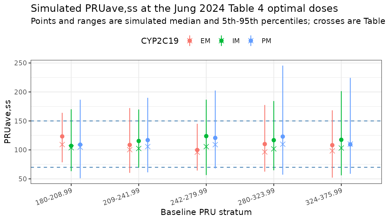
Replicates Jung 2024 Figure 3. The qualitative conclusions all reproduce: the required dose rises with baseline PRU within every phenotype, and the dose ratios versus EM are those the paper reports.
| Baseline PRU stratum | EM | IM | PM | IM / EM | PM / EM |
|---|---|---|---|---|---|
| 180-208.99 | 30 | 60 | 120 | 2.00 | 4.00 |
| 209-241.99 | 45 | 75 | 150 | 1.67 | 3.33 |
| 242-279.99 | 60 | 90 | 180 | 1.50 | 3.00 |
| 280-323.99 | 75 | 120 | 240 | 1.60 | 3.20 |
| 324-375.99 | 90 | 150 | 300 | 1.67 | 3.33 |
Assumptions and deviations
-
Koutuses the unrounded 0.00576, not Table 2’s printed 0.006. Only the unrounded value reproduces the paper’s own derived baseline of 212.67 PRU and its stated 5-day turnover half-life; the rounded value gives 204.17 and 4.81 days. Results ‘PD submodel’ states the unrounded value explicitly. -
The IIV column of Table 2 is read as standard
deviations. The column is headed “Standard deviation” and
Results ‘PD submodel’ calls the
Emaxvalue of 0.501 “the standard deviation (omega)”, so theini()block records each variance as the square of the tabulated value. -
The paper’s Delta-method IIV percentages for
fm1andfm2do not reproduce. Results ‘PK submodel’ reports coefficients of variation of 24.52 / 26.44 / 27.78% (fm1) and 2.78 / 11.13 / 27.87% (fm2) across EM / IM / PM. Neither the first-order Delta approximationCV = (1 - p) * omeganor an exact simulation from the logit-normal reproduces these from omega = 0.255 and 1.130, under either a standard-deviation or a variance reading of the tabulated values. These percentages are a derived summary, not a model input, so the packaged model uses the tabulated omegas directly; the discrepancy is flagged here rather than resolved by adjusting any value. -
Baseline PRU is an input in the dose-optimization
simulations. The five strata span 180-376 PRU, which the
reported
Kinvariability could not generate (reaching 350 PRU would require a 4-sigma random effect). Baseline is therefore sampled inside each stratum and mapped ontoKinviabaseline = Kin / Kout, replacing rather than supplementing theKinrandom effect. The paper does not state its mechanism, but its statement thatPRUave,ssvariability shows a “positive dependence … on baseline PRU levels” is consistent with this reading, and the reportedKinomega of 0.120 matches the observed baseline CV of 11.4% in the trial cohort, i.e. it describes the trial’s own baseline spread. -
Parameter uncertainty is not reproduced. The paper
simulated by “random sampling from the estimated parameter-covariance
matrix”, but only per-parameter %RSEs are published, not the covariance
matrix. This is the most likely cause of the two residual discrepancies
above: the simulated
PRUave,ssdistribution here is narrower than Table S1’s (5th percentiles near 57 versus the paper’s near 49), and the proportion inside the 70-150 window is correspondingly a few points higher. The typical-value medians sit about 4% above Table S1 on average. Extending treatment far beyond three weeks changes the typical-value result by under 0.1%, so incomplete convergence to steady state is not the explanation. -
Predicted H4 concentrations exceed the stated assay
calibration range. The typical-value single-dose H4 Cmax is
about 116 ng/mL, above the 0.3-50 ng/mL H4 calibration range given in
Methods, whereas the parent (3.1 ng/mL against 0.09-10) and the
carboxylic acid (2474 ng/mL against 50-5000) both fall inside theirs.
This follows directly from the paper’s own reported values through the
identity
AUCinf(H4) = 1.106 * fm1 * fm2 * Dose / CLm1, which involves no volume and no inter-compartmental term, so it is a property of the published parameter set rather than of this transcription. It is also what makes the reportedEC50of 67.32 ng/mL an on-scale quantity: were H4 confined below 50 ng/mL, the sigmoid would never approach half-maximal effect. Samples above the upper limit of quantification are routinely diluted and re-assayed, which would reconcile the two statements, but the paper does not say so. -
fmothersis not carried as a state. The1 - fm2share of the hepatic metabolic flux goes to unmeasured metabolites and appears only as the part ofCLcnot routed into either metabolite compartment, exactly as in the paper’s equations. -
VHis not an independent parameter. Methods ‘PK model’ sets the hepatic volume equal to the central volume because the two were not separately identifiable, sovh <- vcinmodel()and theVcrandom effect propagates to both. -
The
(1 - fm1) * fm2split is confirmed three independent ways. Methods ‘PK model’, the printeddAm2/dtequation, and the Table 3 footnote all givefmcarbo = (1 - fm1) * fm2, and Table 3’s numbers agree ((1 - 0.125) * 0.960 = 0.840). Worth stating explicitly because a two-column text extraction of the PDF displaces the parentheses onto their own line, making the expression look like1 - fm1 * fm2, which would give 0.880 instead and match nothing in the paper. -
No demographic covariates. The paper screened
weight, age, height, albumin, creatinine, AST, ALT, alkaline
phosphatase, gamma-GT, total bilirubin, blood urea nitrogen and total
protein and retained none; these are recorded in the model file’s
covariatesDataExcludedso the screen’s provenance is preserved without declaring unused covariates. - No published NCA table exists, so the PKNCA section is validated against exposure identities derived from the paper’s own differential equations rather than against tabulated Cmax / AUC values.
- Cohort sizes are smaller than the paper’s. Jung 2024 used 1000 virtual subjects per subgroup; this vignette uses 150 per phenotype arm for the profile figure and 100 per subgroup for the 15-cell dose-optimization grid, to stay inside the package’s simulation-size and render-time budgets.
-
Metabolite naming. The carboxylic acid metabolite
uses the previously registered
clocasuffix (founded byPejcic_2024_clopidogrel.R), so this model’s states arecentral_clocaandperipheral1_cloca. The active thiol uses the registeredh4suffix (founded byDanielak_2017_clopidogrel.R). The platelet-reactivity state is the newly registeredprucompartment withPRUas its observation output, following the existinganc/ANCpairing.