Lormetazepam (le Noble 2024)
Source:vignettes/articles/leNoble_2024_lormetazepam.Rmd
leNoble_2024_lormetazepam.RmdModel and source
- Citation: le Noble JLML, Shudofsky KN, Foudraine N, Punt N, Janssen PKJ. Pharmacokinetics of Enteral Lormetazepam in Mechanically Ventilated ICU Patients with COVID-19: An Adjunct Sedative Study. Clin Pharmacokinet. 2024;63(12):1769-1776. doi:10.1007/s40262-024-01455-3. PMCID PMC11649707. Parameter estimates from main-text Table 2; full-precision estimates and the population covariance matrix from Electronic Supplementary Material Part 1 (KinPop output of the final model ‘1-POP-All’, ‘Cycles = 118’).
- Description: One-compartment population pharmacokinetic model with first-order absorption for enteral (nasogastric) lormetazepam in mechanically ventilated ICU adults with COVID-19-associated ARDS (le Noble 2024), developed by an iterative two-stage Bayesian procedure in Edsim++/KinPop. Apparent volume scales linearly and apparent clearance allometrically (exponent 0.75) with body weight per 70 kg. Correlated inter-individual variability on Ka, V/F and CL/F; proportional residual error. Creatinine clearance and CRP were screened and not retained.
- Article: https://doi.org/10.1007/s40262-024-01455-3 (open access, PMC11649707)
- Supplementary information: Electronic Supplementary Material Part 1 (the Edsim++/KinPop output of the final model, with goodness-of-fit plots) and Part 2 (the bootstrap run), available with the article.
Population
Fifteen critically ill adults on invasive mechanical ventilation for severe COVID-19-associated acute respiratory distress syndrome were studied at VieCuri Medical Center (Venlo, the Netherlands) between 9 and 20 April 2020. All were ventilated in the prone position with PaO2/FiO2 below 200. Eighteen patients had residual blood samples; three on continuous veno-venous hemofiltration were excluded. Table 1 reports 11 men and 4 women (27% female), age mean 61.6 years (SD 13), height median 172.0 cm (IQR 163.5-180.5), ICU-admission BMI median 29.1 kg/m^2 (IQR 27.4-31.1), APACHE IV median 57 (IQR 55-68), serum creatinine median 70 umol/L (IQR 58.5-83), creatinine clearance median 79 mL/min (IQR 64-114) and CRP median 164 mg/L (IQR 113.5-210.5). Body weight is used in the model but no weight summary is reported.
Lormetazepam 2 mg was given twice daily (08:00 and 20:00) through a nasogastric tube as an adjunct to intravenous propofol, midazolam and dexmedetomidine. Residual arterial samples from routine draws at 06:30, 16:00 and 22:00 were assayed by UHPLC-MS/MS (1-20 ug/L); the median was ten samples per patient (range 2-21), and the population fit used 116 concentrations (Supplement Part 1). Concentrations below the limit of quantitation were excluded.
The same information is recorded in the model’s
population metadata.
Model structure
A one-compartment model with first-order absorption, fitted by the iterative two-stage Bayesian method of the KinPop plugin of Edsim++ 2.4. The apparent volume is reported per 70 kg and the apparent clearance per 70 kg^0.75 (Table 2 units), so
ka = Ka
V  = V/F_70  * (WT / 70)
CL = CL/F_70 * (WT / 70)^0.75
Cc = 1000 * A_central / V          (ug/L, dose in mg)
The residual error is proportional. Creatinine clearance and CRP were tested by linear regression against the individual clearances (Figures 1 and 2) and not retained.
Source trace
| Model element | Value | Source |
|---|---|---|
| One-compartment, first-order absorption | – | Methods, Pharmacokinetic Model Development; Results, Population Pharmacokinetic Compartmental Analysis |
| V/F per 70 kg, linear in weight |
e_wt_vc fixed 1 |
Table 2 unit ‘L/70 kg’ |
| CL/F per 70 kg^0.75 |
e_wt_cl fixed 0.75 |
Table 2 unit ‘L/h/70 kg0.75’ |
lka |
6.3778 1/h | Table 2 Ka 6.4; Supplement Part 1 PO.k |
lvc |
207.3061 L/70 kg | Table 2 V/F 207; Supplement Part 1 C01.V |
lcl |
14.5041 L/h/70 kg^0.75 | Table 2 CL/F 14.5; Supplement Part 1 TE.CL |
etalka |
CV 152.5% -> 1.201666 | Table 2 CV% 153; Supplement Part 1 ‘Pop’ covariance 2.33 |
etalvc |
CV 50.6% -> 0.227660 | Table 2 CV% 51; Supplement Part 1 ‘Pop’ covariance 0.256 |
etalcl |
CV 50.0% -> 0.223433 | Table 2 CV% 50; Supplement Part 1 ‘Pop’ covariance 0.250 |
| Ka-V, Ka-CL, V-CL covariances | 0.051179, -0.073280, 0.102789 | Supplement Part 1 ‘Pop’ correlations 0.0681, -0.0926, 0.4279 |
propSd |
0.4931 | Table 2 ‘Prop’ 49%; Supplement Part 1 SD.Sd1 |
The KinPop covariance matrix in Supplement Part 1 is printed relative
to the parameter means: its diagonal is the squared CV (0.506^2 = 0.256,
1.525^2 = 2.33, 0.500^2 = 0.250). Each element is converted to the log
scale of the log-normal parameters by
omega_ij = log(1 + rho_ij * CV_i * CV_j).
mod <- readModelDb("leNoble_2024_lormetazepam")
ui <- rxode2::rxode(mod)
#> ℹ parameter labels from comments will be replaced by 'label()'

cv <- c(ka = 9.7262 / 6.3778, vc = 104.8195 / 207.3061, cl = 7.2573 / 14.5041)
rho <- matrix(
  c(1, 0.0681, -0.0926,
    0.0681, 1, 0.4279,
    -0.0926, 0.4279, 1),
  3,
  dimnames = list(names(cv), names(cv))
)
rel_cov <- rho * outer(cv, cv)
omega_expected <- log(1 + rel_cov)
omega_model <- ui$omega[c("etalka", "etalvc", "etalcl"), c("etalka", "etalvc", "etalcl")]

# The relative covariances reproduce the printed 'Pop' values (2.33, 0.256,
# 0.250 on the diagonal; 0.0525, -0.0706, 0.108 off it) to their printed
# three significant figures, and the model omega matches the conversion to
# the six decimals written in the model file.
stopifnot(
  max(abs(rel_cov[c(1, 5, 9)] / c(2.33, 0.256, 0.250) - 1)) < 0.005,
  max(abs(rel_cov[c(2, 3, 6)] / c(0.0525, -0.0706, 0.108) - 1)) < 0.005,
  max(abs(omega_model - omega_expected)) < 1e-6
)
knitr::kable(omega_model, digits = 6, caption = "Log-scale IIV covariance matrix carried in the model.")| etalka | etalvc | etalcl | |
|---|---|---|---|
| etalka | 1.201666 | 0.051179 | -0.073280 |
| etalvc | 0.051179 | 0.227660 | 0.102789 |
| etalcl | -0.073280 | 0.102789 | 0.223433 |
Replicate Figure 3: alternative dosing regimens
Figure 3 shows typical-patient simulations of three regimens chosen with the Edsim++ dose-calculation plugin to give a steady-state trough of 6 ug/L: 0.92 mg q8h, 1.62 mg q12h and 5.36 mg q24h, each continued to about 144 h and followed to 180 h. The figure does not state the simulated body weight. With the published population means carried as typical values, a 70 kg patient reproduces the 6 ug/L trough of every regimen, which is the check below.
mod_typical <- rxode2::zeroRe(mod)
#> ℹ parameter labels from comments will be replaced by 'label()'

regimens <- data.frame(
  regimen = c("5.36 mg q24h", "1.62 mg q12h", "0.92 mg q8h"),
  dose = c(5.36, 1.62, 0.92),
  tau = c(24, 12, 8),
  last_dose = c(120, 132, 136),
  # Steady-state peaks digitised by the maintainers from Figure 3.
  peak_digitised = c(30.3, 13.1, 9.9)
)

fig3_events <- function(dose, tau, last_dose, id) {
  dose_times <- seq(0, last_dose, by = tau)
  obs_times <- sort(unique(c(seq(0, 180, by = 0.05), dose_times)))
  dplyr::bind_rows(
    data.frame(id = id, time = dose_times, evid = 1L, amt = dose, cmt = "depot"),
    data.frame(id = id, time = obs_times, evid = 0L, amt = NA_real_, cmt = "central")
  ) |>
    dplyr::mutate(WT = 70) |>
    dplyr::arrange(time, dplyr::desc(evid))
}

ev_fig3 <- dplyr::bind_rows(lapply(seq_len(nrow(regimens)), function(i) {
  fig3_events(regimens$dose[i], regimens$tau[i], regimens$last_dose[i], i)
}))

sim_fig3 <- rxode2::rxSolve(mod_typical, ev_fig3, rtol = 1e-10, atol = 1e-12) |>
  as.data.frame() |>
  dplyr::mutate(regimen = factor(regimens$regimen[id], levels = regimens$regimen))
#> ℹ omega/sigma items treated as zero: 'etalka', 'etalvc', 'etalcl'
#> Warning: multi-subject simulation without without 'omega'
ggplot(sim_fig3, aes(time, Cc)) +
  geom_line(colour = "blue") +
  geom_hline(yintercept = c(6, 16), linetype = "dashed", colour = "red") +
  facet_wrap(~regimen, ncol = 1) +
  scale_x_continuous(breaks = seq(0, 180, by = 12)) +
  coord_cartesian(ylim = c(0, 35)) +
  labs(x = "Time (h)", y = "Lormetazepam concentration (ug/L)")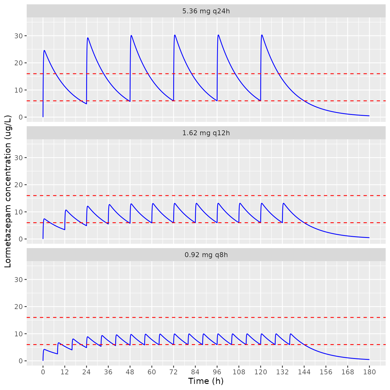
Replicates Figure 3 of le Noble 2024: typical-patient (70 kg) concentrations for the three alternative regimens; dashed lines mark the 6-16 ug/L therapeutic range.
The steady-state trough is read just before the last dose, and the steady-state peak is the maximum over the dosing interval that ends there. The published peaks were digitised by the maintainers from Figure 3 (about 30, 13 and 10 ug/L for the q24h, q12h and q8h panels).
fig3_check <- sim_fig3 |>
  dplyr::mutate(regimen = as.character(regimen)) |>
  dplyr::left_join(regimens, by = "regimen") |>
  dplyr::group_by(regimen) |>
  dplyr::summarise(
    trough_ss = Cc[time == last_dose[1]][1],
    peak_ss = max(Cc[time >= last_dose[1] - tau[1] & time <= last_dose[1]]),
    peak_digitised = peak_digitised[1],
    .groups = "drop"
  ) |>
  dplyr::mutate(trough_published = 6)

fig3_check |>
  dplyr::rename(
    "Regimen" = regimen,
    "Simulated trough (ug/L)" = trough_ss,
    "Target trough (ug/L)" = trough_published,
    "Simulated peak (ug/L)" = peak_ss,
    "Figure 3 peak, digitised (ug/L)" = peak_digitised
  ) |>
knitr::kable(digits = 2, caption = "Steady state of the Figure 3 regimens at 70 kg.")| Regimen | Simulated trough (ug/L) | Simulated peak (ug/L) | Figure 3 peak, digitised (ug/L) | Target trough (ug/L) |
|---|---|---|---|---|
| 0.92 mg q8h | 5.98 | 9.94 | 9.9 | 6 |
| 1.62 mg q12h | 6.01 | 13.16 | 13.1 | 6 |
| 5.36 mg q24h | 5.99 | 30.29 | 30.3 | 6 |
# Deterministic typical-value solve. The dose-calculation plugin chose each
# dose for a 6 ug/L trough and printed it to two decimals (about 0.3% of
# 1.62 mg), so 2% admits the rounding while a wrong reference weight
# (80 kg gives troughs of 5.5-5.6) or a median-for-mean reading of the
# parameters (troughs of 6.75) fails.
stopifnot(
  nrow(fig3_check) == 3L,
  max(abs(fig3_check$trough_ss / 6 - 1)) < 0.02,
  max(abs(fig3_check$peak_ss / fig3_check$peak_digitised - 1)) < 0.05
)
The typical half-life at 70 kg is 9.91 h; the paper reports a median individual half-life of 10.7 h (IQR 8.7-12.4).
Virtual cohort
The study regimen, 2 mg every 12 h via nasogastric tube, is simulated for 200 virtual patients over five days. Body weight is not summarised in the paper, so it is built from Table 1: height normal with median 172.0 cm and the SD implied by the IQR (17 / 1.349 = 12.6 cm, kept within 150-200 cm), ICU BMI normal with median 29.1 kg/m^2 and SD 3.7 / 1.349 = 2.74 (kept within 20-45), and weight = BMI x height^2. Out-of-range draws are redrawn.
set.seed(20240411)
rxode2::rxSetSeed(20240411)

n_sub <- 200L

draw_truncated <- function(n, mean, sd, lower, upper) {
  x <- rnorm(n, mean, sd)
  bad <- x < lower | x > upper
  while (any(bad)) {
    x[bad] <- rnorm(sum(bad), mean, sd)
    bad <- x < lower | x > upper
  }
  x
}

cohort <- data.frame(
  id = seq_len(n_sub),
  height_cm = draw_truncated(n_sub, 172.0, 12.6, 150, 200),
  bmi = draw_truncated(n_sub, 29.1, 2.74, 20, 45)
) |>
  dplyr::mutate(WT = bmi * (height_cm / 100)^2)

summary(cohort$WT)
#>    Min. 1st Qu.  Median    Mean 3rd Qu.    Max.
#>   55.58   77.55   86.64   87.77   98.23  125.28
dose_times <- seq(0, 108, by = 12)
obs_times <- sort(unique(c(seq(0, 120, by = 0.25), 108 + c(0.1, 0.2, 0.3, 0.4, 0.5, 0.6, 0.7, 0.8, 0.9))))

ev_cohort <- dplyr::bind_rows(
  tidyr::expand_grid(id = cohort$id, time = dose_times) |>
    dplyr::mutate(evid = 1L, amt = 2, cmt = "depot"),
  tidyr::expand_grid(id = cohort$id, time = obs_times) |>
    dplyr::mutate(evid = 0L, amt = NA_real_, cmt = "central")
) |>
  dplyr::left_join(dplyr::select(cohort, id, WT), by = "id") |>
  dplyr::arrange(id, time, dplyr::desc(evid)) |>
  dplyr::mutate(treatment = "2 mg q12h")

sim <- rxode2::rxSolve(mod, ev_cohort, keep = "treatment") |>
  as.data.frame()
#> ℹ parameter labels from comments will be replaced by 'label()'

stopifnot(!anyNA(sim$Cc))
sim |>
  dplyr::group_by(time) |>
  dplyr::summarise(
    p05 = quantile(Cc, 0.05),
    p50 = median(Cc),
    p95 = quantile(Cc, 0.95),
    .groups = "drop"
  ) |>
  ggplot(aes(time, p50)) +
  geom_ribbon(aes(ymin = p05, ymax = p95), fill = "steelblue", alpha = 0.3) +
  geom_line(colour = "steelblue4") +
  geom_hline(yintercept = c(6, 16), linetype = "dashed", colour = "red") +
  scale_x_continuous(breaks = seq(0, 120, by = 12)) +
  labs(x = "Time (h)", y = "Lormetazepam concentration (ug/L)")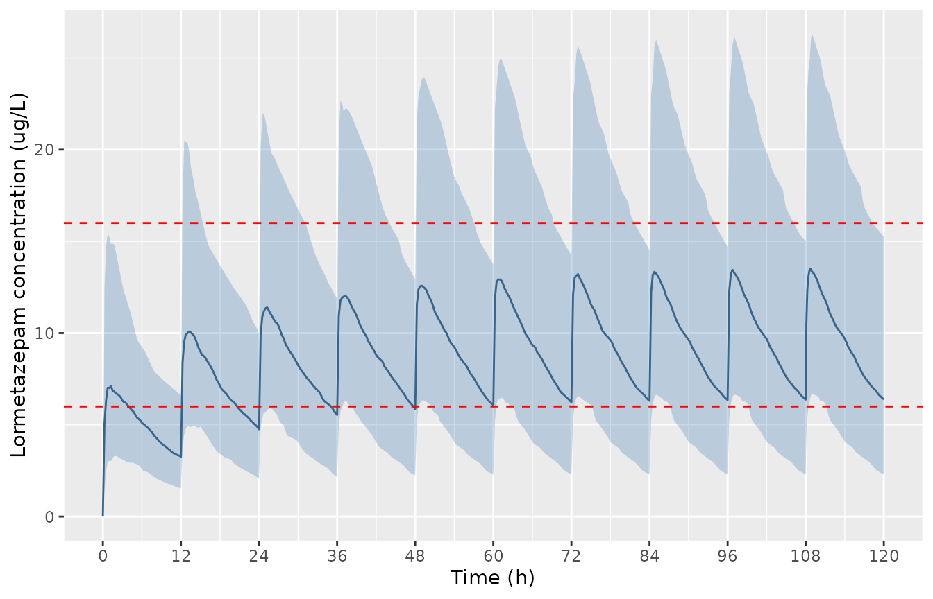
Simulated concentrations over five days of 2 mg q12h: median and 5th-95th percentile band of the individual predictions (no residual error) for 200 virtual patients.
PKNCA validation
Non-compartmental analysis of the individual predictions (no residual error) over the fifth-day dosing interval, 108-120 h.
conc_df <- sim |>
  dplyr::filter(time >= 108, !is.na(Cc)) |>
  dplyr::select(id, time, Cc, treatment)

dose_df <- ev_cohort |>
  dplyr::filter(evid == 1L, time == 108) |>
  dplyr::select(id, time, amt, treatment)

conc_obj <- PKNCA::PKNCAconc(conc_df, Cc ~ time | treatment + id)
dose_obj <- PKNCA::PKNCAdose(dose_df, amt ~ time | treatment + id)

intervals <- data.frame(
  start = 108,
  end = 120,
  cmax = TRUE,
  tmax = TRUE,
  cmin = TRUE,
  auclast = TRUE,
  half.life = TRUE
)

nca_res <- PKNCA::pk.nca(PKNCA::PKNCAdata(conc_obj, dose_obj, intervals = intervals))
summary(nca_res)
#>  start end treatment   N    auclast        cmax        cmin                tmax
#>    108 120 2 mg q12h 200 117 [47.8] 13.6 [42.8] 6.12 [69.1] 0.600 [0.100, 4.50]
#>    half.life
#>  12.0 [5.73]
#>
#> Caption: auclast, cmax, cmin: geometric mean and geometric coefficient of variation; tmax: median and range; half.life: arithmetic mean and standard deviation; N: number of subjects
Comparison against the published values
The paper reports medians from its individual compartmental analysis of the observed 2 mg q12h data (Results, “Individual Pharmacokinetic Compartmental Analysis”): Cmax 10.93 ug/L (IQR 10.28-11.67), trough 5.48 ug/L (IQR 4.12-5.97), Tmax 0.64 h (IQR 0.6-0.7) and half-life 10.7 h (IQR 8.7-12.4). These are per-patient fits, not the population model, and the patients were sampled at varying times in their course, so they are not a steady-state NCA of the population model. They are compared below as a plausibility check.
reference <- data.frame(
  treatment = "2 mg q12h",
  cmax = 10.93,
  cmin = 5.48,
  tmax = 0.64,
  half.life = 10.7
)

cmp <- nlmixr2lib::ncaComparisonTable(
  nca_res,
  reference,
  by = "treatment",
  units = c(cmax = "ug/L", cmin = "ug/L", tmax = "h", half.life = "h")
)
knitr::kable(cmp, caption = "Simulated steady-state NCA (median of 200 virtual patients) against the paper's individual-analysis medians.")| NCA parameter | treatment | Reference | Simulated | % diff |
|---|---|---|---|---|
| Cmax (ug/L) | 2 mg q12h | 10.9 | 13.7 | +25.0%* |
| Cmin (ug/L) | 2 mg q12h | 5.48 | 6.37 | +16.3% |
| Tmax (h) | 2 mg q12h | 0.64 | 0.6 | -6.3% |
| t½ (h) | 2 mg q12h | 10.7 | 10.8 | +0.5% |
if (!is.null(attr(cmp, "footnote"))) cat(attr(cmp, "footnote"), "\n")
#> * differs from reference by more than ±20%.

nca_long <- as.data.frame(nca_res$result)
sim_median <- function(code) median(nca_long$PPORRES[nca_long$PPTESTCD == code], na.rm = TRUE)

# Cohort medians against individual-analysis medians. Realised ratios
# 1.25 (Cmax), 1.16 (trough) and 1.01 (half-life) at 1 and 8 threads; the
# Monte Carlo SE of a 200-subject median with 50% CV is about 4%, so the
# bounds sit at least 3 SE outside the realised values. A dropped
# mg/L -> ug/L factor (1000-fold) or a 2-fold error in V/F or CL/F still
# breaks them.
stopifnot(
  abs(sim_median("cmax") / 10.93 - 1) < 0.45,
  abs(sim_median("cmin") / 5.48 - 1) < 0.35,
  abs(sim_median("half.life") / 10.7 - 1) < 0.25
)
The simulated steady-state trough is 16% above, and the half-life within 1% of, the reported medians. The simulated Cmax is about 25% above the reported median 10.93 ug/L and is flagged in the table. The simulated Cmax and Tmax are summarised from a dense post-dose grid, whereas the paper’s medians come from individual fits to sparse routine samples (06:30, 16:00 and 22:00, never within 1.5 h of a dose), so the absorption phase was poorly informed in the data; the paper’s Discussion attributes the 153% CV on Ka to this. The typical 70 kg patient on 2 mg q12h has a steady-state peak of about 16 ug/L (Figure 3 scaled by 2 / 1.62), so the population model itself predicts peaks above the individual-analysis median; the difference is not a transcription error.
Assumptions and deviations
-
Mean read as typical value. KinPop reports each
log-normal parameter as a population mean +/- SD. The mean is carried as
the typical value (the log-normal median) and the CV converted by
omega^2 = log(1 + CV^2), as in the other Edsim++/KinPop and MwPharm models in the package (Meenks_2023_flucloxacillin,Daskapan_2019_darunavir,Geers_2022_clozapine). Figure 3 supports this reading: at 70 kg it reproduces the 6 ug/L trough of all three regimens, whereas reading the mean as the arithmetic mean of the log-normal (typical value = mean / sqrt(1 + CV^2)) gives troughs of about 6.75 ug/L. -
IIV correlations included. Table 2 prints only the
CVs; the full population covariance matrix and correlations are from
Supplement Part 1 and are carried as an
etalka + etalvc + etalclblock. -
Full-precision estimates. Values are taken at the
precision of the Supplement Part 1 output (
Cycles = 118); Table 2 prints the same values rounded. - Proportional residual error. Table 2 labels the residual ‘Prop’; the KinPop output marks SD.Sd1 with ‘Log: Yes’. It is encoded as proportional.
-
Bioavailability. Not identifiable from enteral data
alone; V/F and CL/F are apparent and the dose enters
depotwithout an F term. - Body weight. Weight is a model covariate but the paper gives no weight summary. The virtual cohort derives weight from the Table 1 height and BMI medians and IQRs, assuming normal distributions; the Figure 3 replication uses 70 kg, the reference weight of the parameters.
-
Screened covariates. Creatinine clearance and CRP
are recorded in
covariatesDataExcluded; neither enters the model. - Lormetazepam glucuronide. The metabolite was assayed and summarised as a metabolic ratio (median 11.5, not MW-corrected) but was not modelled; the package model describes lormetazepam only.