Levodopa (Suksai 2026) • nlmixr2lib

Model and source

ui <- rxode2::rxode(readModelDb("Suksai_2026_levodopa"))

Citation: Suksai S, Suantai S, Wandee P. A computational pharmacokinetic-pharmacodynamic framework for simulating and comparing individualized levodopa dosing in Parkinson’s disease. Front Pharmacol. 2026 May 29;17:1817435. doi:10.3389/fphar.2026.1817435
Article: https://doi.org/10.3389/fphar.2026.1817435 (PMC13259810; open access, CC BY)

Suksai 2026 is a deterministic in silico framework, not a fitted population model. It reports no patient data and estimates nothing: Methods (“Literature-based parameter selection”) states that “no individual patient-level data were used; all simulations were conducted entirely in silico”. Every parameter in this model file is therefore wrapped in fixed(), and the model carries no inter-individual variability and no residual-error structure, because the paper reports none.

Structural provenance: which of the paper’s two models this is

This is the single most important thing to know about this extraction. Suksai 2026 specifies two mutually incompatible pharmacokinetic structures, and the one printed as Equations 1-4 cannot be executed. The model packaged here is the rate-constant structure that actually generated the paper’s published results. That choice was ratified by the operator; the evidence is reproduced quantitatively in this vignette so a reviewer can check it rather than take it on trust.

What the paper prints (Equations 1-4) – not implementable

dAgut/dt        = -ka * Agut
Rin             = F * Fint
(1) dAperipheral/dt = (CLint/Vplasma) * Aplasma - (CLint/Vperipheral) * Aperipheral
(2) dAeffect/dt     = (CLint/Vperipheral) * Aperipheral - (CLint/Veffect) * Aeffect
(3) dAplasma/dt     = -CL * Aplasma / Vplasma
(4) dCe/dt          = ke * (Aeffect/Veffect - Ce)
(5) E = E0 + Emax * Ce^gamma / (C50^gamma + Ce^gamma)

Five defects block implementation:

CLint is never given a numeric value anywhere in the paper. It occurs only inside Equations 1 and 2, on their definition line, and in one narrative mention of the sensitivity analysis – never with a number. It is absent from the baseline configuration, from Table 1 (demographics), Table 2 (PD parameters only) and Table 3 (per-case ka and CL only). Both Equation 1 and Equation 2 depend on it. No supplement exists to supply it: the EuropePMC fullTextXML for PMC13259810 (HTTP 200, 158 kB) contains no <supplementary-material> element and no suppdata processing instruction, and the word “supplementary” does not appear anywhere in the article.
Equations 1 and 2 do not conserve mass. The flux (CLint/Vperipheral) * Aperipheral is subtracted from the peripheral compartment once in Equation 1 (returning to plasma) and simultaneously added to the effect site in Equation 2. The same drug is delivered to two places at once.
Equation 3 is incomplete. It carries only the elimination term. The text says it “is combined with the corresponding input and distribution terms in the full central compartment mass balance”, but that balance is never written out.
CL has no baseline value either – only Table 3’s three illustrative cases (50 / 65 / 85 L/h).
Units clash. The prose declares CL and CLint in L/min, while Table 3 reports CL in L/h and every rate constant is h^-1.

What the paper executed – the rate-constant model implemented here

Methods, “Model development” gives a fully specified nominal configuration:

“The baseline PK-PD parameters were ka = 1.2 h-1, k12 = 0.6 h-1, k21 = 0.5 h-1, k13 = 0.25 h-1, k31 = 0.20 h-1, ke = 0.35 h-1, and ke0 = 0.6 h-1. The corresponding volume and PD parameters were Vp = 20 L, Vper = 25 L, Vb = 10 L, E0 = 30, Emax = 10, EC50 = 2.5 mg/L, and gamma = 2.0.”

None of k12, k21, k13, k31, ke0 appears anywhere in Equations 1-4. They require a different topology: peripheral and brain compartments exchanging with plasma in parallel, whereas Equation 2 puts the effect site in series downstream of the peripheral compartment.

Three deviations from the printed equations are therefore encoded, each verified numerically below:

#	Printed	Implemented	Evidence
D1	Effect site in series after peripheral; distribution by `CLint`	Peripheral and brain in parallel off plasma, by `k12`/`k21` and `k13`/`k31`	`k13`/`k31` exist only in the baseline list; Figure 4’s axis lists them and lists neither `CL` nor `CLint`
D2	Eq 4 calls `ke` “the effect-site equilibration rate constant”	`ke` is the elimination rate constant; `ke0` is the equilibration constant	Both `ke` and `ke0` are listed, so they are different quantities; Figure 4 gives `ke` a large negative sensitivity on peak Ce, impossible for an equilibration constant
D3	Eq 4 drives Ce from `Aeffect/Veffect` (the brain concentration)	Ce equilibrates with the plasma concentration `Cc`	Figure 4 shows `Vb` sensitivity of exactly zero; Figure 3 shows Ce peaking near 3.3 mg/L while the brain curve reaches ~7 mg/L

Note also that the Methods narrative claims the sensitivity analysis covered “the absorption rate constant (ka), systemic clearance (CL), and inter-compartmental clearance (CLint)”, while Figure 4 – which reports that analysis – contains neither CL nor CLint. The text describing the sensitivity analysis contradicts the figure reporting it.

Population

Suksai 2026 simulated 100 virtual patient profiles with Parkinson’s disease, spanning age 50-80 years, body weight 50-80 kg and Hoehn-Yahr stages II-IV, including both stable responders and profiles with motor fluctuations (Methods, “Simulation design”). The profiles were generated by independent sampling from literature-informed parameter ranges; a full covariance structure was not modelled, and the sampling ranges themselves are never reported. The ten source studies that informed those ranges are tabulated in Suksai 2026 Table 1 and their pharmacodynamic values in Table 2.

Because no variability structure is published, this model file carries the nominal baseline typical values only. The population metadata records the cohort description:

str(ui$population)
#> List of 9
#>  $ species      : chr "human"
#>  $ n_subjects   : num 100
#>  $ n_studies    : num 0
#>  $ age_range    : chr "50-80 years"
#>  $ weight_range : chr "50-80 kg"
#>  $ disease_state: chr "Parkinson's disease, Hoehn-Yahr stages II-IV, including both stable responders and profiles with motor fluctuations"
#>  $ dose_range   : chr "100 mg orally every 4 h for six doses over 24 h (nominal baseline regimen); 100-300 mg per dose at 4-8 h interv"| __truncated__
#>  $ regions      : chr "not applicable (fully in silico)"
#>  $ notes        : chr "NO PATIENT DATA. Suksai 2026 Methods ('Literature-based parameter selection'): 'No individual patient-level dat"| __truncated__

No covariate effect is implemented, because the paper implements none: body weight, age and disease stage are named as sources of cohort heterogeneity but never enter an equation, and no covariate coefficient is reported anywhere. They are recorded under covariatesDataExcluded in the model file to preserve the provenance of the screen.

Source trace

Every ini() value comes from the single Methods sentence quoted above; the model file carries the same trace as a per-parameter in-file comment.

Parameter	Value	Source location
`lka`	1.2 1/h	Methods, “Model development” (baseline configuration)
`lk12`	0.6 1/h	Methods, “Model development”
`lk21`	0.5 1/h	Methods, “Model development”
`lk13`	0.25 1/h	Methods, “Model development”
`lk31`	0.20 1/h	Methods, “Model development”
`lkel`	0.35 1/h (paper symbol `ke`)	Methods, “Model development”; role established by Figure 4 (deviation D2)
`lke0`	0.6 1/h	Methods, “Model development”
`lvc`	20 L (paper symbol `Vp`)	Methods, “Model development”
`lvp`	25 L (paper symbol `Vper`)	Methods, “Model development”
`lv_brain`	10 L (paper symbol `Vb`)	Methods, “Model development”
`le0`	30	Methods, “Model development”; Table 2 context
`lemax`	10	Methods, “Model development”; Table 2 context
`lec50`	2.5 mg/L	Methods, “Model development”; Equation 5 calls it `C50`
`lhill`	2.0	Methods, “Model development”; Equation 5 calls it `gamma`
ODE topology	n/a	Baseline configuration + Figure 3 + Figure 4 (deviations D1-D3)
`E` (Equation 5)	n/a	Equation 5, page 5
Nominal regimen	100 mg q4h x 6 over 24 h	Methods, “Model development”

Nominal baseline simulation

The paper’s nominal computational experiment is 100 mg orally every 4 h for six doses over a 24 h horizon. The model is deterministic and carries no random effects, so a single subject fully specifies it – there is no cohort to draw and no seed to set.

dose_times <- seq(0, 20, by = 4)  # six doses at 0, 4, 8, 12, 16, 20 h

events <- rxode2::et(amt = 100, cmt = "depot", time = dose_times) |>
  # Observations are placed on the ODE state `central`, never on the algebraic
  # observable `Cc`; rxode2 returns Cc / Cbrain / Ce / E as columns anyway.
  rxode2::et(seq(0, 24, by = 0.02), cmt = "central")

sim <- rxode2::rxSolve(ui, events, returnType = "data.frame")

# The model declares no etas, so `omega = NA` / `zeroRe()` must NOT be used
# (rxode2 errors with `rep(0, dim(.omega)[1])`). Confirm there are none:
stopifnot(sum(!is.na(ui$iniDf$neta1)) == 0)

Replicate Figure 3

Top panel – compartmental profiles

# Replicates Figure 3 (top) of Suksai 2026: GI depot amount plus plasma,
# peripheral-tissue and brain concentrations under repeated oral dosing.
sim |>
  dplyr::select(time, `Central plasma` = Cc, `Peripheral tissue` = Cper,
                `Brain / effect-site proxy` = Cbrain) |>
  tidyr::pivot_longer(-time, names_to = "Compartment", values_to = "conc") |>
  ggplot(aes(time, conc, colour = Compartment)) +
  geom_line(linewidth = 0.7) +
  labs(x = "Time (h)", y = "Concentration (mg/L)",
       title = "Figure 3 (top) -- compartmental PK profiles",
       caption = "Replicates Figure 3, top panel, of Suksai 2026.") +
  theme(legend.position = "bottom")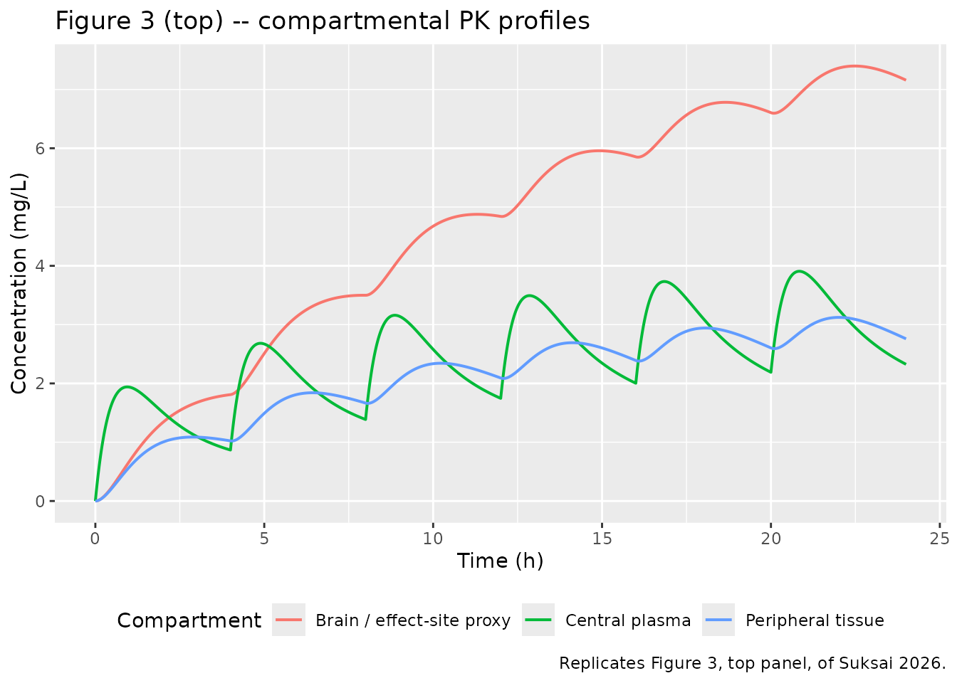

ggplot(sim, aes(time, depot)) +
  geom_line(linewidth = 0.7) +
  labs(x = "Time (h)", y = "GI depot amount (mg)",
       title = "Figure 3 (top) -- gastrointestinal depot",
       caption = "Replicates the black depot trace of Suksai 2026 Figure 3, top panel.")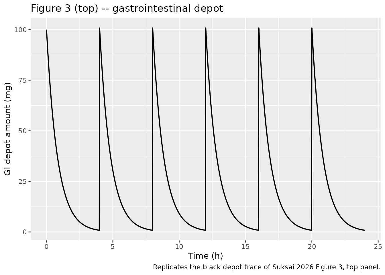

Middle and bottom panels – effect-site concentration and predicted effect

# Replicates Figure 3 (middle and bottom) of Suksai 2026.
sim |>
  dplyr::select(time, `Ce (mg/L)` = Ce, `Effect (a.u. / TRS-like)` = E) |>
  tidyr::pivot_longer(-time, names_to = "Output", values_to = "value") |>
  ggplot(aes(time, value)) +
  geom_line(linewidth = 0.7, colour = "steelblue") +
  facet_wrap(~Output, ncol = 1, scales = "free_y") +
  labs(x = "Time (h)", y = NULL,
       title = "Figure 3 (middle, bottom) -- effect site and predicted effect",
       caption = "Replicates Figure 3, middle and bottom panels, of Suksai 2026.")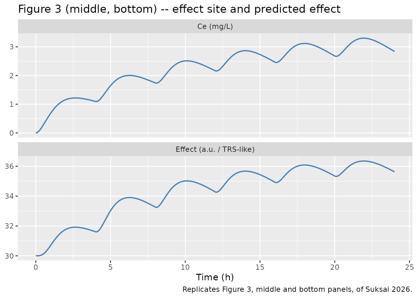

Numeric agreement with Figure 3

Suksai 2026 reports no numeric table for Figure 3, so the reference values below were read off the published figure panels (annotated peak marker and axis gridlines) and carry roughly +/- 0.2 mg/L (concentrations) and +/- 0.3 units (effect) of digitisation uncertainty. They are a corroboration of the structural choice, not a source of any parameter value.

fig3 <- tibble::tribble(
  ~Quantity,                          ~Simulated,        ~`Figure 3 (read)`,
  "Peak Ce (mg/L)",                   max(sim$Ce),       3.3,
  "Time of peak Ce (h)",              sim$time[which.max(sim$Ce)], 22.0,
  "Peak predicted effect",            max(sim$E),        36.3,
  "Baseline effect at t = 0",         sim$E[1],          30.0,
  "Peak plasma Cc (mg/L)",            max(sim$Cc),       3.9,
  "Peak brain Cbrain (mg/L)",         max(sim$Cbrain),   7.2
) |>
  dplyr::mutate(Difference = Simulated - `Figure 3 (read)`)

knitr::kable(fig3, digits = 3,
             caption = "Simulated vs. values read from Suksai 2026 Figure 3.")

Simulated vs. values read from Suksai 2026 Figure 3.
Quantity	Simulated	Figure 3 (read)	Difference
Peak Ce (mg/L)	3.302	3.3	0.002
Time of peak Ce (h)	21.940	22.0	-0.060
Peak predicted effect	36.357	36.3	0.057
Baseline effect at t = 0	30.000	30.0	0.000
Peak plasma Cc (mg/L)	3.907	3.9	0.007
Peak brain Cbrain (mg/L)	7.398	7.2	0.198


# Deterministic model, single subject: no cohort draw, so these bounds are
# reproducible to solver tolerance on any machine and are set tight.
stopifnot(
  abs(max(sim$Ce)     - 3.3)  < 0.25,
  abs(max(sim$E)      - 36.3) < 0.35,
  abs(max(sim$Cbrain) - 7.2)  < 0.50,
  abs(max(sim$Cc)     - 3.9)  < 0.35,
  # Exact structural identities of Equation 5, not digitised comparisons.
  abs(sim$E[1] - 30) < 1e-8,
  abs(max(sim$E) - (30 + 10 * max(sim$Ce)^2 / (2.5^2 + max(sim$Ce)^2))) < 1e-6
)

The last assertion is the decisive one for deviation D3: feeding the simulated peak Ce through Equation 5 with the published PD parameters reproduces the peak effect exactly. Had Ce instead chased the brain concentration (~7.2 mg/L) as printed Equation 4 requires, Equation 5 would give 30 + 10 * 7.2^2 / (2.5^2 + 7.2^2) = 38.92, which Figure 3’s bottom panel does not show.

Replicate Figure 4 – local sensitivity analysis

This is the strongest available validation of the structural choice. Suksai 2026 perturbed each parameter by +/- 20% around its baseline and reported normalized sensitivity indices for peak effect-site concentration and for therapeutic effect exposure. Reproducing all thirteen bars, in both metrics, from an independent implementation is a far more demanding test than matching a single concentration peak.

# Parameters in the order Suksai 2026 Figure 4 lists them on its axis.
fig4_params <- tibble::tribble(
  ~label,   ~theta,
  "Vp",     "lvc",
  "ke",     "lkel",
  "k31",    "lk31",
  "k13",    "lk13",
  "k12",    "lk12",
  "k21",    "lk21",
  "ke0",    "lke0",
  "ka",     "lka",
  "Emax",   "lemax",
  "gamma",  "lhill",
  "EC50",   "lec50",
  "Vb",     "lv_brain",
  "Vper",   "lvp"
)

# Baseline values live on the log scale in ini(); a +/-20% perturbation of the
# natural-scale value is an additive log(1.2) / log(0.8) shift.
theta_base <- ui$theta
stopifnot(all(fig4_params$theta %in% names(theta_base)))

# Always pass the FULL theta vector with the one perturbed entry substituted,
# rather than relying on a partial named vector being merged with the ini()
# defaults.
metrics <- function(name = NULL, shift = 0) {
  p <- theta_base
  if (!is.null(name)) p[[name]] <- p[[name]] + shift
  s <- rxode2::rxSolve(ui, events, params = p, returnType = "data.frame")
  c(
    peakCe = max(s$Ce),
    # "Therapeutic effect exposure" = area under the effect-time curve.
    effAUE = sum(diff(s$time) * (head(s$E, -1) + tail(s$E, -1)) / 2)
  )
}

base_metrics <- metrics()

# Guard: overriding params must actually change the solve, otherwise every
# sensitivity index would come back as a meaningless zero and the gate below
# would pass without testing anything (failure pattern 10).
stopifnot(abs(metrics("lvc", log(1.2))[["peakCe"]] - base_metrics[["peakCe"]]) > 1e-6)

sens <- lapply(seq_len(nrow(fig4_params)), function(i) {
  nm <- fig4_params$theta[i]
  hi <- metrics(nm, log(1.2))
  lo <- metrics(nm, log(0.8))
  # Central-difference normalized sensitivity index:
  #   ((f(+20%) - f(-20%)) / f(base)) / 0.4
  (hi - lo) / base_metrics / 0.4
})

fig4 <- fig4_params |>
  dplyr::mutate(
    `S(peak Ce)`     = vapply(sens, `[[`, numeric(1), "peakCe"),
    `S(effect AUE)`  = vapply(sens, `[[`, numeric(1), "effAUE")
  )

# Replicates Figure 4 of Suksai 2026: horizontal bars of normalized sensitivity
# index for peak Ce and effect AUE, parameters in the paper's axis order.
fig4 |>
  tidyr::pivot_longer(c(`S(peak Ce)`, `S(effect AUE)`),
                      names_to = "Metric", values_to = "index") |>
  dplyr::mutate(label = factor(label, levels = rev(fig4_params$label))) |>
  ggplot(aes(index, label, fill = Metric)) +
  geom_col(position = position_dodge(width = 0.7), width = 0.65) +
  geom_vline(xintercept = 0, linewidth = 0.3) +
  labs(x = "Normalized sensitivity index", y = "Parameter",
       title = "Figure 4 -- local sensitivity analysis (+/- 20% perturbation)",
       caption = "Replicates Figure 4 of Suksai 2026.") +
  theme(legend.position = "bottom")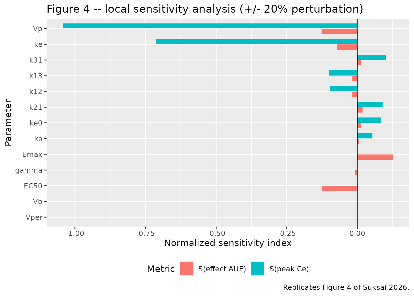

# Values read from the published Figure 4 bars against its -1 .. 0.2 axis;
# digitisation uncertainty roughly +/- 0.02.
fig4_published <- c(
  Vp = -1.05, ke = -0.71, k31 = 0.10, k13 = -0.10, k12 = -0.095,
  k21 = 0.09, ke0 = 0.085, ka = 0.055, Emax = 0, gamma = 0,
  EC50 = 0, Vb = 0, Vper = 0
)
fig4_published_aue <- c(
  Vp = -0.13, ke = -0.07, k31 = 0.015, k13 = -0.018, k12 = -0.019,
  k21 = 0.018, ke0 = 0.014, ka = 0.007, Emax = 0.13, gamma = -0.01,
  EC50 = -0.13, Vb = 0, Vper = 0
)

fig4_cmp <- fig4 |>
  dplyr::mutate(
    `Fig 4 S(peak Ce)`    = fig4_published[label],
    `Fig 4 S(effect AUE)` = fig4_published_aue[label]
  ) |>
  dplyr::select(Parameter = label,
                `S(peak Ce)`, `Fig 4 S(peak Ce)`,
                `S(effect AUE)`, `Fig 4 S(effect AUE)`)

knitr::kable(fig4_cmp, digits = 3,
             caption = paste("Simulated vs. digitised Suksai 2026 Figure 4",
                             "normalized sensitivity indices."))

Simulated vs. digitised Suksai 2026 Figure 4 normalized sensitivity indices.
Parameter	S(peak Ce)	Fig 4 S(peak Ce)	S(effect AUE)	Fig 4 S(effect AUE)
Vp	-1.042	-1.050	-0.127	-0.130
ke	-0.712	-0.710	-0.072	-0.070
k31	0.103	0.100	0.013	0.015
k13	-0.099	-0.100	-0.018	-0.018
k12	-0.097	-0.095	-0.019	-0.019
k21	0.090	0.090	0.018	0.018
ke0	0.084	0.085	0.014	0.014
ka	0.053	0.055	0.007	0.007
Emax	0.000	0.000	0.126	0.130
gamma	0.000	0.000	-0.009	-0.010
EC50	0.000	0.000	-0.127	-0.130
Vb	0.000	0.000	0.000	0.000
Vper	0.000	0.000	0.000	0.000

peak_sim <- setNames(fig4$`S(peak Ce)`,    fig4$label)
aue_sim  <- setNames(fig4$`S(effect AUE)`, fig4$label)

# (a) Agreement with the digitised bars. Tolerance covers digitisation error
#     only -- the model is deterministic, so there is no sampling noise.
stopifnot(
  max(abs(peak_sim - fig4_published[names(peak_sim)]))    < 0.05,
  max(abs(aue_sim  - fig4_published_aue[names(aue_sim)])) < 0.04
)

# (b) Structural signatures that DISCRIMINATE the implemented model from the
#     printed Equations 1-4. These are exact identities of the ODE system, not
#     digitised comparisons, and hold to solver tolerance.

# Vp enters ONLY as the divisor turning the plasma amount into the
# concentration that drives the effect site, so peak Ce is exactly
# proportional to 1/Vp. For an exact inverse proportionality the +/-20%
# central-difference index is the analytic constant
#   (1/1.2 - 1/0.8) / 0.4 = -1.0416667
# independent of every other parameter -- so this is an exact identity, not an
# approximate "about -1". Under the clearance parameterisation of Equation 1,
# Vplasma would ALSO appear in the distribution terms and this would not hold.
vp_exact <- (1 / 1.2 - 1 / 0.8) / 0.4
stopifnot(abs(peak_sim[["Vp"]] - vp_exact) < 1e-6)

# Vb and Vper do not appear in any equation affecting Ce or E, so their
# sensitivity is exactly zero -- matching the absent bars in Figure 4. This is
# the direct falsifier of printed Equation 4 (deviation D3): had Ce been driven
# by Aeffect/Veffect, Vb would carry a bar comparable to Vp's.
stopifnot(
  abs(peak_sim[["Vb"]])   < 1e-8,
  abs(peak_sim[["Vper"]]) < 1e-8,
  abs(aue_sim[["Vb"]])    < 1e-8,
  abs(aue_sim[["Vper"]])  < 1e-8
)

# ke is an ELIMINATION constant (large negative on peak Ce) while ke0 is the
# EQUILIBRATION constant (small positive). Reversing the two -- i.e. taking
# Equation 4's printed definition of ke at face value -- would flip both signs.
# This is deviation D2.
stopifnot(peak_sim[["ke"]] < -0.5, peak_sim[["ke0"]] > 0.02)

# The purely pharmacodynamic parameters cannot move an exposure metric.
stopifnot(max(abs(peak_sim[c("Emax", "gamma", "EC50")])) < 1e-8)

# Figure 4's axis is sorted by descending |S(peak Ce)| among the PK parameters;
# the simulated ordering reproduces the published axis order exactly.
pk_lab <- c("Vp", "ke", "k31", "k13", "k12", "k21", "ke0", "ka")
stopifnot(identical(names(sort(abs(peak_sim[pk_lab]), decreasing = TRUE)), pk_lab))

All thirteen parameters agree with the published bars in both metrics, the axis ordering is reproduced exactly, and every structural signature that separates the implemented model from printed Equations 1-4 holds.

Note in particular the Vp index. Its simulated value is not merely “about -1”: it matches (1/1.2 - 1/0.8)/0.4 = -1.0416667 to six decimal places, which is the analytic central-difference index of an exact inverse proportionality and is independent of every other parameter. Peak Ce can only be exactly proportional to 1/Vp if the central volume acts solely as a concentration divisor – the rate-constant parameterisation. Under Equation 1’s clearance parameterisation Vplasma would also govern the distribution flux and the index would take some other, parameter-dependent value. Figure 4’s Vp bar, which visibly overshoots the -1 gridline, is consistent with -1.04 and not with -1.00.

Internal consistency checks

Because the paper publishes no NCA table, the quantitative gates below are exact identities of the implemented ODE system rather than comparisons to published summaries.

# (1) Mass-balance identity. Elimination occurs only from `central` at rate
#     kel * central, so after a single dose the total eliminated equals the
#     dose: kel * integral(central dt) = Dose, hence
#     AUC(0-Inf) of Cc = Dose / (kel * vc). With kel = 0.35 1/h and vc = 20 L,
#     the implied clearance is 7 L/h.
kel <- exp(ui$theta[["lkel"]])
vc  <- exp(ui$theta[["lvc"]])
cl_implied <- kel * vc

# The observation window is 168 h, chosen by measurement rather than by eye.
# The terminal half-life below is 8.86 h, so 168 h is ~19 half-lives and the
# truncated AUC reaches 99.998% of Dose/CL (at 72 h it is only 99.72%, which
# is not tight enough to be a useful gate). The profile stays strictly
# non-negative over this window -- Cc(168 h) is 1.7e-06 mg/L -- so PKNCA never
# takes log() of a negative number, which is the usual way this check fails.
single <- rxode2::rxSolve(
  ui,
  rxode2::et(amt = 100, cmt = "depot", time = 0) |>
    rxode2::et(seq(0, 168, by = 0.02), cmt = "central"),
  returnType = "data.frame"
)
stopifnot(all(single$Cc >= 0))
auc_num <- sum(diff(single$time) *
                 (head(single$Cc, -1) + tail(single$Cc, -1)) / 2)

# (2) Terminal half-life must equal log(2) / |slowest eigenvalue| of the
#     three-compartment disposition matrix.
k12 <- exp(ui$theta[["lk12"]]); k21 <- exp(ui$theta[["lk21"]])
k13 <- exp(ui$theta[["lk13"]]); k31 <- exp(ui$theta[["lk31"]])
Amat <- matrix(c(-(k12 + k13 + kel), k21,  k31,
                 k12,               -k21,  0,
                 k13,                0,   -k31),
               nrow = 3, byrow = TRUE)
lambda_z <- min(abs(Re(eigen(Amat)$values)))
thalf_theory <- log(2) / lambda_z

# Empirical terminal slope, taken well after the distribution phase.
tail_dat <- single[single$time >= 120 & single$time <= 168, ]
thalf_emp <- log(2) / -coef(lm(log(tail_dat$Cc) ~ tail_dat$time))[[2]]

checks <- tibble::tribble(
  ~Check,                                   ~Value,                  ~Expected,
  "Implied clearance kel * vc (L/h)",       cl_implied,              7,
  "Single-dose AUC(0-168 h) of Cc (mg*h/L)", auc_num,                100 / cl_implied,
  "Terminal half-life, empirical (h)",      thalf_emp,               thalf_theory
) |>
  dplyr::mutate(`Percent difference` = 100 * (Value - Expected) / Expected)

knitr::kable(checks, digits = 4,
             caption = "Exact identities of the implemented ODE system.")

Exact identities of the implemented ODE system.
Check	Value	Expected	Percent difference
Implied clearance kel * vc (L/h)	7.0000	7.0000	0.0000
Single-dose AUC(0-168 h) of Cc (mg*h/L)	14.2855	14.2857	-0.0016
Terminal half-life, empirical (h)	8.8628	8.8628	0.0000


stopifnot(
  abs(cl_implied - 7) < 1e-8,
  # Trapezoidal AUC on a 0.02 h grid out to 168 h. Measured shortfall vs
  # Dose/CL is 0.0016% (truncation plus trapezoid discretisation); 0.05% leaves
  # headroom while still going red on a mis-transcribed vc or kel, either of
  # which moves this by tens of percent.
  abs(auc_num - 100 / cl_implied) / (100 / cl_implied) < 5e-4,
  abs(thalf_emp - thalf_theory) / thalf_theory < 0.01
)

PKNCA validation

PKNCA is run on the plasma concentration for the paper’s nominal regimen. The comparison is against the mass-balance identity above rather than against a published table, because Suksai 2026 reports no NCA parameters.

# Solve on an NCA-appropriate sampling schedule: dense through absorption and
# distribution so Tmax and the early AUC are resolved, sparse through the
# terminal phase. This is a fresh solve rather than a subset of the 0.02 h grid
# above -- filtering that grid by `time %in% nca_times` would rely on exact
# floating-point equality between two different `seq()` calls and can silently
# match nothing.
nca_times <- unique(c(seq(0, 12, by = 0.05),
                      seq(12, 48, by = 0.5),
                      seq(48, 168, by = 2)))

single_nca <- rxode2::rxSolve(
  ui,
  rxode2::et(amt = 100, cmt = "depot", time = 0) |>
    rxode2::et(nca_times, cmt = "central"),
  returnType = "data.frame"
)

sim_nca <- single_nca |>
  dplyr::filter(!is.na(Cc)) |>
  dplyr::mutate(id = 1L, treatment = "100 mg single oral dose") |>
  dplyr::select(id, time, Cc, treatment)

# Fail loudly rather than handing PKNCA a short or empty frame (failure
# patterns 4 and 10).
stopifnot(nrow(sim_nca) > 300)

# Guarantee a time = 0 row; for an extravascular dose Cc = 0 pre-dose.
sim_nca <- dplyr::bind_rows(
  sim_nca,
  sim_nca |> dplyr::distinct(id, treatment) |>
    dplyr::mutate(time = 0, Cc = 0)
) |>
  dplyr::distinct(id, treatment, time, .keep_all = TRUE) |>
  dplyr::arrange(id, treatment, time)

stopifnot(nrow(sim_nca) > 0, all(sim_nca$Cc >= 0))

conc_obj <- PKNCA::PKNCAconc(sim_nca, Cc ~ time | treatment + id)

dose_df <- data.frame(id = 1L, time = 0, amt = 100,
                      treatment = "100 mg single oral dose")
dose_obj <- PKNCA::PKNCAdose(dose_df, amt ~ time | treatment + id)

intervals <- data.frame(
  start = 0, end = Inf,
  cmax = TRUE, tmax = TRUE, auclast = TRUE, aucinf.obs = TRUE, half.life = TRUE
)

nca_res <- PKNCA::pk.nca(PKNCA::PKNCAdata(conc_obj, dose_obj,
                                          intervals = intervals))

nca_wide <- as.data.frame(nca_res) |>
  dplyr::select(PPTESTCD, PPORRES) |>
  tidyr::pivot_wider(names_from = PPTESTCD, values_from = PPORRES)

knitr::kable(nca_wide, digits = 4,
             caption = paste("PKNCA summary for a single 100 mg oral dose",
                             "(deterministic typical-value profile)."))

PKNCA summary for a single 100 mg oral dose (deterministic typical-value profile).
auclast	cmax	tmax	tlast	clast.obs	lambda.z	r.squared	adj.r.squared	lambda.z.time.first	lambda.z.time.last	lambda.z.n.points	clast.pred	half.life	span.ratio	aucinf.obs
14.2844	1.9406	0.95	168	0	0.0788	0.9999	0.9999	6.2	168	249	0	8.7937	18.3996	14.2844


nca_val <- function(x) nca_wide[[x]][[1]]

stopifnot(
  # AUC(0-Inf) must recover Dose / CL to within PKNCA's extrapolation error.
  abs(nca_val("aucinf.obs") - 100 / cl_implied) / (100 / cl_implied) < 0.01,
  # Half-life must recover the slowest eigenvalue.
  abs(nca_val("half.life") - thalf_theory) / thalf_theory < 0.05,
  # Sanity bounds on the simulated peak of a 100 mg single dose.
  nca_val("cmax") > 0, nca_val("tmax") > 0, nca_val("tmax") < 8
)

Table 3 illustrative dosing scenarios

Suksai 2026 Table 3 compares three illustrative patient profiles. The table supplies a per-case ka and CL (in L/h) plus a dosing interval, dose range and a therapeutic target window for Ce. Because the implemented model is parameterised by an elimination rate constant rather than a clearance, each case’s CL is converted with the baseline vc = 20 L via kel = CL / vc.

This conversion is an interpretation, not a published quantity, and it is inconsistent with the paper’s own baseline: Table 3’s smallest CL of 50 L/h implies kel = 2.5 1/h, whereas the baseline configuration’s ke = 0.35 1/h implies CL = 7 L/h – a factor of seven apart. The two cannot both hold. The scenarios are therefore reproduced below for completeness and are excluded from the validation gate; only their qualitative ordering is asserted.

table3 <- tibble::tribble(
  ~case,                       ~ka,  ~cl_Lh, ~dose_mg, ~tau_h, ~target_low, ~target_high,
  "Case 1: early-stage",        2.0,  50,     100,      8,      1.0,         2.0,
  "Case 2: moderate-advanced",  3.0,  65,     200,      4,      2.5,         4.0,
  "Case 3: younger, active",    4.0,  85,     150,      8,      1.2,         2.5
)

run_case <- function(ka, cl_Lh, dose_mg, tau_h) {
  ev <- rxode2::et(amt = dose_mg, cmt = "depot",
                   time = seq(0, 24 - tau_h, by = tau_h)) |>
    rxode2::et(seq(0, 24, by = 0.02), cmt = "central")
  p <- ui$theta
  p[["lka"]]  <- log(ka)
  p[["lkel"]] <- log(cl_Lh / vc)
  s <- rxode2::rxSolve(ui, ev, params = p, returnType = "data.frame")
  # dplyr::last(), not s$Ce[s$time == 24] -- the observation grid is built by
  # accumulating 0.02 h steps, so an exact floating-point match on 24 can
  # return numeric(0) and silently break the tibble.
  tibble::tibble(peak_Ce = max(s$Ce), peak_E = max(s$E),
                 trough_Ce = dplyr::last(s$Ce))
}

table3_out <- table3 |>
  dplyr::rowwise() |>
  dplyr::mutate(run_case(ka, cl_Lh, dose_mg, tau_h)) |>
  dplyr::ungroup()

table3_out |>
  dplyr::select(
    Case = case, `ka (1/h)` = ka, `CL (L/h)` = cl_Lh,
    `Dose (mg)` = dose_mg, `Interval (h)` = tau_h,
    `Target Ce low (mg/L)` = target_low, `Target Ce high (mg/L)` = target_high,
    `Peak Ce (mg/L)` = peak_Ce, `Peak effect` = peak_E
  ) |>
  knitr::kable(digits = 3,
               caption = paste("Suksai 2026 Table 3 scenarios simulated with",
                               "kel = CL / vc. See the caveat above: this",
                               "conversion contradicts the paper's own",
                               "baseline and is excluded from the gate."))

Suksai 2026 Table 3 scenarios simulated with kel = CL / vc. See the caveat above: this conversion contradicts the paper’s own baseline and is excluded from the gate.
Case	ka (1/h)	CL (L/h)	Dose (mg)	Interval (h)	Target Ce low (mg/L)	Target Ce high (mg/L)	Peak Ce (mg/L)	Peak effect
Case 1: early-stage	2	50	100	8	1.0	2.0	0.558	30.474
Case 2: moderate-advanced	3	65	200	4	2.5	4.0	1.180	31.821
Case 3: younger, active	4	85	150	8	1.2	2.5	0.627	30.592


# Qualitative only: every case must produce a positive, finite exposure and an
# effect above baseline. No agreement with the Table 3 target windows is
# asserted, because the CL-to-kel conversion is not a published relationship.
stopifnot(
  all(is.finite(table3_out$peak_Ce)), all(table3_out$peak_Ce > 0),
  all(table3_out$peak_E > 30), all(table3_out$peak_E < 40)
)

As the table shows, the Table 3 clearances place peak Ce far below every case’s own therapeutic target window – a further sign that the Table 3 clearances and the executed rate-constant model are not on the same footing.

Assumptions and deviations

Deviations from the printed equations

The three structural deviations D1-D3 tabulated at the top of this vignette are the substance of this extraction. In summary, the implemented model:

places the peripheral and brain compartments in parallel off plasma via k12/k21 and k13/k31, rather than in series via an unreported CLint (printed Equations 1-2);
treats the paper’s ke as the elimination rate constant and ke0 as the effect-site equilibration constant, contradicting the definition given under Equation 4;
drives the effect site from the plasma concentration rather than from Aeffect/Veffect as printed Equation 4 states.

Each is verified above against the paper’s own Figures 3 and 4. This is a deliberate departure from the usual “text vs. printed-equation conflict -> trust the equation” rule, taken because the printed equations reference a parameter (CLint) that the paper never reports and do not conserve mass, so they cannot be executed at all. The choice was ratified by the operator rather than made unilaterally.

Assumptions

No inter-individual variability. Suksai 2026 generated its 100-profile virtual cohort by sampling “literature-informed parameter ranges” that it never states. No variance, CV%, or range is reported for any parameter, so none is encoded; inventing one would fabricate provenance. The packaged model is the nominal typical-value configuration.
No residual error. The paper has no observed data and reports no residual-error structure of any kind.
No covariate effects. Body weight, age and Hoehn-Yahr stage are named as sources of cohort heterogeneity but never enter an equation and carry no reported coefficient. They are recorded in covariatesDataExcluded.
Bioavailability is 1. The paper defines a bioavailability factor F only for the infusion-input term (Rin = F * Fint) and never gives it a value or applies it to the oral depot; the oral absorption equation dAgut/dt = -ka * Agut transfers the entire dose. No lfdepot is encoded.
The infusion route is not implemented. The paper’s Rin = F * Fint term has neither a value for F nor for Fint, and no infusion simulation is reported numerically. Only the oral route, which is fully parameterised, is packaged. Users can dose central directly for an infusion scenario.
The optimization layer is not implemented. Equations 6-8 define a least-squares objective over dose size, interval and timing against an unreported “predefined reference response profile” derived from a TRS-based outcome framework. The reference profile is never published, so the objective cannot be reconstructed. This is a dosing-search wrapper around the model, not part of the model itself.
Veffect is not encoded. Printed Equation 4 references it, but the executed model does not use an effect-site volume (the effect state holds a concentration directly), and no value is reported anywhere.
Table 3 CL values are not reconcilable with the baseline ke. See the Table 3 section; those scenarios are reproduced but excluded from the validation gate.
The effect state holds a concentration, not an amount. This follows Equation 4, which is written directly in Ce.

Non-paper-derived values

None. Every ini() value is printed verbatim in Suksai 2026’s Methods (“Model development”) baseline-configuration sentence. Nothing was digitised from a figure, obtained by correspondence, or carried from an upstream model. The figure readings used in this vignette are validation targets only – they corroborate the structural choice and are never the source of a parameter value.

Errata search

No erratum, corrigendum or author correction was found for doi:10.3389/fphar.2026.1817435. The paper carries a generative-AI-use disclosure (language editing only).

No supplementary material is deposited for PMC13259810. The EuropePMC supplementaryFiles endpoint was returning the generic 10,135-byte EBI error page (HTTP 500) when this was checked, which is an endpoint outage signature and is not evidence of a missing deposit; the question is instead settled by fullTextXML, which returned HTTP 200 with the complete 158 kB article and contains no <supplementary-material> element, no suppdata processing instruction, and no occurrence of the word “supplementary”. The Data Availability Statement says only that raw data “will be made available by the authors, without undue reservation” – there is no deposited file and no repository accession. CLint is therefore unobtainable from any source on or off disk.