Molnupiravir (Bihorel 2023)
Source:vignettes/articles/Bihorel_2023_molnupiravir.Rmd
Bihorel_2023_molnupiravir.RmdModel and source
- Citation: Bihorel S, Cao Y, Chawla A, Birger R, Maas BM, Gao W, Roepcke S, Sardella S, Humphrey R, Kondragunta S, Jayaraman B, Martinho M, Painter W, Painter G, Holman W, De Anda C, Brown ML, Johnson MG, Paschke A, Rizk ML, Stone JA. Population pharmacokinetics of molnupiravir in adults with COVID-19: Lack of clinically important exposure variation across individuals. CPT Pharmacometrics Syst Pharmacol. 2023 Dec;12(12):1859-1871. doi:10.1002/psp4.13031. PMCID: PMC10725262.
- Description: Two-compartment population PK model with Savic transit-compartment absorption and linear elimination for plasma beta-D-N4-hydroxycytidine (NHC), the circulating active nucleoside of the orally administered prodrug molnupiravir (MK-4482, EIDD-2801), in 1207 healthy adults and adults with COVID-19 pooled across one phase I, two phase II and one phase II/III trial (Bihorel 2023). Doses and concentrations are in molar units (molnupiravir 329.31 Da, NHC 259.2 Da). Absorption is an Erlang transit chain (NN = 7.84 compartments, mean transit time MTT = 0.435 h in the fasted-capsule reference) feeding a depot that empties first-order at ka = 0.797 1/h; MTT is raised 422% by a high-fat meal and lowered 61.6% for the oral solution relative to the capsule, neither of which alters the extent of absorption (relative bioavailability F1 fixed at 1). Apparent elimination clearance CL/F = 70.6 L/h in an 80 kg participant rises less-than-proportionally with body weight (power 0.412); apparent central volume Vc/F = 63.9 L in a man of BMI 28 kg/m2 rises with BMI (power 0.997) and is 33% lower in women. Interindividual variability is carried on CL/F (43.4% CV) and Vc/F (62.9% CV); the mean transit time carries inter-occasion variability (39.8% CV) over two occasions rather than IIV. Proportional residual error is stratified by trial phase (25.5% CV for the densely sampled phase I trial, 49.7% CV for the sparsely sampled phase II/III trials). No covariate effect moved the AUC(0-12) geometric mean ratio outside the 0.7-2.0 clinical comparability bounds, so no dose adjustment is recommended for any subpopulation studied.
- Article: https://doi.org/10.1002/psp4.13031
Molnupiravir (MK-4482, EIDD-2801) is an orally administered
ribonucleoside prodrug. It is essentially undetectable in plasma because
it is hydrolysed to beta-D-N4-hydroxycytidine (NHC) during absorption
and first pass, so NHC is the analyte that was measured and modelled.
Bihorel 2023 converted all dose amounts to molar units with the
molnupiravir molecular mass (329.31 Da) and all concentrations with the
NHC molecular mass (259.2 Da); the packaged model keeps those units, so
an 800 mg dose enters as 800 / 329.31 * 1e6 = 2,429,322
nmol and Cc is in nmol/L.
Population
The analysis pooled 4202 plasma NHC concentrations from 1207 participants in four randomised, double-blind, placebo-controlled trials (Bihorel 2023 Table 1): the phase I trial MK-4482-004 in 100 healthy adults, the phase IIa trial MK-4482-006 in 66 non-hospitalised participants with COVID-19, the phase II trial MOVe-IN (MK-4482-001) in 196 hospitalised participants, and the phase II/III trial MOVe-OUT (MK-4482-002) in 845 non-hospitalised participants. Overall 48.3% were women, median (range) age was 46 (18-91) years, median body weight 85 (36.1-172) kg and median BMI 30.4 (14.3-68.6) kg/m^2. Two thirds (66.7%) were White. Renal impairment was common (48.1% mild, 7.0% moderate); hepatic impairment, graded with a modified Child-Pugh score approximated from bilirubin and albumin, was rare (5.0% mild, 0.2% moderate).
Sampling was highly unbalanced: healthy participants contributed 7-26
samples each while participants with COVID-19 contributed 1-5, so 72.8%
of the pooled population contributed at most two samples. That imbalance
is why the model carries two proportional residual-error magnitudes,
selected by STUDY_MOV_PHASE23.
The same information is available programmatically via
readModelDb("Bihorel_2023_molnupiravir")()$population.
Source trace
Every value below is also recorded as an in-file comment beside its
ini() entry in
inst/modeldb/specificDrugs/Bihorel_2023_molnupiravir.R.
| Equation / parameter | Value | Source location |
|---|---|---|
lka |
0.797 1/h | Table 2, row “k a / First-order absorption rate constant, 1/h” (RSE 2.57%) |
lmtt |
0.435 h | Table 2, row “MTT / Mean absorption transit time, h” (RSE 5.39%) |
nn |
7.84 | Table 2, row “NN / Number of transit compartments” (RSE 16.5%) |
e_highfat_mtt |
4.22 | Table 2, row “Proportional shift due to high-fat meal” (RSE 6.29%); Results: “422% increase in MTT” |
e_solution_mtt |
-0.616 | Table 2, row “Proportional shift in oral solution” (RSE 5.49%); Results: “61.6% decrease in MTT” |
lfdepot |
fixed at 1 | Table 2, row “F1 / Relative bioavailability” = 1.00, %RSE column reads “Fixed” |
lcl |
70.6 L/h at 80 kg | Table 2, row “CL/F / Apparent central clearance in 80kg participants, L/h” (RSE 1.97%) |
e_wt_cl |
0.412 | Table 2, row “Power of body weight effect” (RSE 14.0%) |
lvc |
63.9 L at BMI 28, male | Table 2, row “V C /F / Apparent central volume in 28kg/m 2 BMI male participants, L” (RSE 5.07%) |
e_bmi_vc |
0.997 | Table 2, row “Power of BMI effect” (RSE 13.1%) |
e_sexf_vc |
-0.330 | Table 2, row “Proportional shift in female participants” (RSE 11.8%) |
lq |
2.99 L/h | Table 2, row “Q/F / Apparent distribution clearance, L/h” (RSE 5.70%) |
lvp |
68.3 L | Table 2, row “V P /F / Apparent peripheral volume, L” (RSE 14.6%) |
etalcl |
0.172573 | Table 2, CL/F variability 43.4 %CV;
log(1 + 0.434^2)
|
etalvc |
0.333371 | Table 2, V C /F variability 62.9 %CV;
log(1 + 0.629^2)
|
etaiov_mtt_1, etaiov_mtt_2
|
0.147049 | Table 2, row “IOV in MTT” 39.8 %CV; log(1 + 0.398^2);
two occasions per the Table 2 note |
propSdPhase1 |
sqrt(0.0652) = 0.255 |
Table 2, “Residual variability / Phase I trials” = 0.0652, 25.5 %CV |
propSdPhase23 |
sqrt(0.247) = 0.497 |
Table 2, “Residual variability / Phase II/III trials” = 0.247, 49.7 %CV |
Absorption structure (transit chain into depot, first-order
ka into central) |
n/a | Figure 1a (stages 1 and 3); Results, “Base model refinement using phase III data” |
| Two-compartment linear disposition | n/a | Abstract; Results, “Base structural model development” |
| Dose / concentration molar conversion | 329.31 and 259.2 Da | Methods, “Bioanalytical methods” |
| Reference individual for the typical profile | 78 kg, BMI 28, man, non-hospitalised | Discussion, paragraph beginning “Simulation of the typical PK profile” |
| Published typical Cmax / Tmax / t1/2 | 11,400 nmol/L, ~1.5 h, 0.6 and 16.5 h | Discussion, same paragraph |
| AUC(0-12) clinical comparability bounds | 23,800-68,000 nmol*h/L | Methods, “Assessment of clinical relevance …” |
| Reference AUC(0-12) used in the NCA comparison | 34,000 nmol*h/L | Derived from the line above by inverting the printed bounds: 23,800 / 0.7 = 68,000 / 2.0 = 34,000 |
Virtual cohort
Original observed data are not publicly available. The simulations below use virtual populations whose covariate distributions approximate the published demographics of Table 1.
DOSE_800MG_NMOL <- 800 / 329.31 * 1e6  # Methods, "Bioanalytical methods"

# Bihorel 2023 Discussion reference individual: a non-hospitalised man of
# 78 kg and BMI 28 kg/m^2 given 800 mg q12h for 5 days (10 doses). Times are
# re-based below so that the LAST dose sits at t = 0, which makes Tmax and the
# terminal half-life unambiguous for PKNCA.
LAST_DOSE_TIME <- 108

ev_typical <- rxode2::et(amt = DOSE_800MG_NMOL, cmt = "depot", ii = 12, addl = 9) |>
  # Observe the ODE state, never the algebraic observable `Cc`.
  rxode2::et(seq(LAST_DOSE_TIME, 240, by = 0.05), cmt = "central") |>
  as.data.frame() |>
  mutate(
    WT = 78, BMI = 28, SEXF = 0,
    FED_HIGHFAT = 0, FORM_SOLUTION = 0,
    OCC = 1, STUDY_MOV_PHASE23 = 0,
    treatment = "Reference individual"
  )
The food-effect and formulation arms below are single 800 mg doses in
the same reference individual, differing only in
FED_HIGHFAT / FORM_SOLUTION. Because both
covariates act solely on the mean transit time and relative
bioavailability is fixed at 1, these arms isolate a pure absorption-rate
effect.
make_single_dose_arm <- function(label, fed_highfat, form_solution, id) {
  rxode2::et(amt = DOSE_800MG_NMOL, cmt = "depot") |>
    rxode2::et(seq(0, 72, by = 0.05), cmt = "central") |>
    as.data.frame() |>
    mutate(
      id = id, WT = 78, BMI = 28, SEXF = 0,
      FED_HIGHFAT = fed_highfat, FORM_SOLUTION = form_solution,
      OCC = 1, STUDY_MOV_PHASE23 = 0,
      treatment = label
    )
}

ev_food <- bind_rows(
  make_single_dose_arm("Capsule, fasted",       0, 0, 1L),
  make_single_dose_arm("Capsule, high-fat meal", 1, 0, 2L),
  make_single_dose_arm("Oral solution, fasted",  0, 1, 3L)
)
stopifnot(!anyDuplicated(unique(ev_food[, c("id", "time", "evid")])))
The stochastic cohort mimics the non-hospitalised phase II/III
population: 200 participants (the per-arm cap), capsules only, with
FED_HIGHFAT drawn from the 25% mixture fraction Bihorel
2023 fixed for participants whose food status was not collected.
N_COHORT <- 200L

# Body weight and BMI are strongly correlated at fixed height; the paper reports
# each marginally (Table 1) but not their correlation, so a bivariate normal with
# rho = 0.8 is assumed and both margins are truncated to the observed ranges.
# See "Assumptions and deviations".
rho <- 0.8
z1 <- rnorm(N_COHORT)
z2 <- rho * z1 + sqrt(1 - rho^2) * rnorm(N_COHORT)
cohort_cov <- tibble(
  id  = seq_len(N_COHORT),
  WT  = pmin(pmax(85.8 + 18.4 * z1, 36.1), 172),   # Table 1 overall mean (SD), range
  BMI = pmin(pmax(30.4 +  6.1 * z2, 14.3), 68.6),  # Table 1 overall mean (SD), range
  SEXF = rbinom(N_COHORT, 1, 0.483),                   # Table 1: 48.3% women
  FED_HIGHFAT = rbinom(N_COHORT, 1, 0.25),             # Results: mixture fraction fixed to 25%
  FORM_SOLUTION = 0,                                   # Table 1: capsules only in phase II/III
  OCC = 1,
  STUDY_MOV_PHASE23 = 1
)

# Coarse grid over the accumulation phase, fine grid over the final interval
# where the NCA is taken.
obs_times <- sort(unique(c(seq(0, 108, by = 0.5), seq(108, 120, by = 0.05))))

ev_template <- rxode2::et(amt = DOSE_800MG_NMOL, cmt = "depot", ii = 12, addl = 9) |>
  rxode2::et(obs_times, cmt = "central") |>
  as.data.frame()
# et() may emit its own single-subject `id`; drop it so `cohort_cov$id` is the
# only subject key.
ev_template$id <- NULL

ev_cohort <- tidyr::crossing(cohort_cov, ev_template) |>
  arrange(id, time, desc(evid))
stopifnot(!anyDuplicated(unique(ev_cohort[, c("id", "time", "evid")])))
Simulation
mod <- readModelDb("Bihorel_2023_molnupiravir")
mod_typical <- rxode2::zeroRe(mod)
#> Warning: some etas defaulted to non-mu referenced, possible parsing error: etaiov_mtt_1, etaiov_mtt_2
#> as a work-around try putting the mu-referenced expression on a simple line
#> Warning: No sigma parameters in the model
#> Warning: some etas defaulted to non-mu referenced, possible parsing error: etaiov_mtt_1, etaiov_mtt_2
#> as a work-around try putting the mu-referenced expression on a simple line

sim_typical <- rxode2::rxSolve(
  mod_typical, events = ev_typical, keep = "treatment",
  omega = NA, sigma = NA, returnType = "data.frame"
)

sim_food <- rxode2::rxSolve(
  mod_typical, events = ev_food, keep = "treatment",
  omega = NA, sigma = NA, returnType = "data.frame"
)

sim_cohort <- rxode2::rxSolve(
  mod, events = ev_cohort, keep = c("WT", "BMI", "SEXF", "FED_HIGHFAT"),
  returnType = "data.frame"
)
#> Warning: some etas defaulted to non-mu referenced, possible parsing error: etaiov_mtt_1, etaiov_mtt_2
#> as a work-around try putting the mu-referenced expression on a simple line
Cc is the individual prediction; residual error appears
in the sim column. The NCA below is deliberately run on
Cc, because the published values being reproduced are model
predictions rather than observations.
Replicate published results
Typical steady-state profile (Discussion)
Bihorel 2023 report that, for the reference individual, “NHC concentration is expected to peak at 11,400 nmol/L ~1.5 h after the last dose, with half-lives of 0.6 and 16.5 h for the first and second phases of disposition.”
sim_typical |>
  mutate(tad = time - LAST_DOSE_TIME) |>
  filter(tad >= 0, tad <= 48) |>
  ggplot(aes(tad, Cc)) +
  geom_line(linewidth = 0.8) +
  geom_hline(yintercept = 11400, linetype = "dashed", colour = "grey40") +
  geom_vline(xintercept = 1.5, linetype = "dashed", colour = "grey40") +
  scale_y_log10() +
  labs(
    x = "Time after the last dose (h)", y = "Plasma NHC (nmol/L)",
    title = "Typical NHC profile after the last of ten 800 mg q12h doses",
    caption = paste(
      "Reference individual: non-hospitalised man, 78 kg, BMI 28 kg/m^2.",
      "Dashed lines mark the published Cmax of 11,400 nmol/L at ~1.5 h",
      "(Bihorel 2023, Discussion)."
    )
  )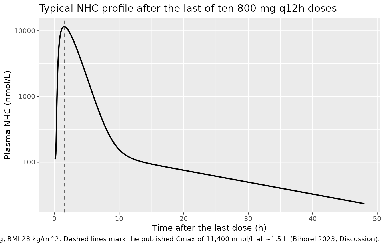
The biexponential decline is a direct consequence of the disposition micro-constants, which can be checked in closed form against the two published half-lives without any simulation at all.
cl_ref  <- 70.6 * (78 / 80)^0.412
vc_ref  <- 63.9
kel <- cl_ref / vc_ref; k12 <- 2.99 / vc_ref; k21 <- 2.99 / 68.3
b <- kel + k12 + k21
d <- sqrt(b^2 - 4 * kel * k21)
hl <- log(2) / c(alpha = (b + d) / 2, beta = (b - d) / 2)

tibble(
  Phase = c("First (alpha)", "Second (beta)"),
  Model = round(unname(hl), 2),
  Published = c(0.6, 16.5)
) |>
  rename("Half-life, model (h)" = Model, "Half-life, published (h)" = Published) |>
knitr::kable(caption = "Disposition half-lives from the model's micro-constants vs Bihorel 2023 Discussion.")| Phase | Half-life, model (h) | Half-life, published (h) |
|---|---|---|
| First (alpha) | 0.61 | 0.6 |
| Second (beta) | 16.54 | 16.5 |
Food and formulation act on absorption rate only
sim_food |>
  filter(time <= 12) |>
  ggplot(aes(time, Cc, colour = treatment)) +
  geom_line(linewidth = 0.8) +
  labs(
    x = "Time (h)", y = "Plasma NHC (nmol/L)", colour = NULL,
    title = "Single 800 mg dose: effect of a high-fat meal and of the oral solution",
    caption = paste(
      "A high-fat meal raises the mean transit time 422% and the oral solution",
      "lowers it 61.6% (Bihorel 2023 Table 2); neither changes the extent of",
      "absorption."
    )
  ) +
  theme(legend.position = "bottom")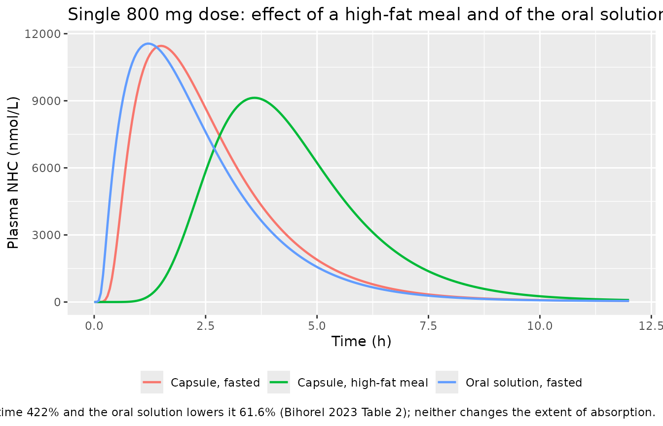
Because FED_HIGHFAT and FORM_SOLUTION act
only on the mean transit time and F1 is fixed at 1, total
exposure must be identical across the three arms. That is an internal
identity of the model rather than a cohort statistic, so it is asserted
tightly.
auc_by_arm <- sim_food |>
  filter(!is.na(Cc)) |>
  group_by(treatment) |>
  summarise(
    auc72 = sum(diff(time) * (head(Cc, -1) + tail(Cc, -1)) / 2),
    cmax = max(Cc), tmax = time[which.max(Cc)], .groups = "drop"
  )

auc_by_arm |>
  rename(
    "Arm" = treatment, "AUC(0-72) (nmol*h/L)" = auc72,
    "Cmax (nmol/L)" = cmax, "Tmax (h)" = tmax
  ) |>
  knitr::kable(digits = c(0, 0, 0, 2),
caption = "Single 800 mg dose by food status and formulation.")| Arm | AUC(0-72) (nmol*h/L) | Cmax (nmol/L) | Tmax (h) |
|---|---|---|---|
| Capsule, fasted | 34690 | 11455 | 1.5 |
| Capsule, high-fat meal | 34683 | 9133 | 3.6 |
| Oral solution, fasted | 34690 | 11556 | 1.2 |
# AUC must be invariant to MTT; only rate changes.
stopifnot(diff(range(auc_by_arm$auc72)) / mean(auc_by_arm$auc72) < 1e-3)
# The high-fat meal must delay and blunt the peak; the solution must sharpen it.
tmax_fasted <- auc_by_arm$tmax[auc_by_arm$treatment == "Capsule, fasted"]
stopifnot(
  auc_by_arm$tmax[auc_by_arm$treatment == "Capsule, high-fat meal"] > tmax_fasted,
  auc_by_arm$tmax[auc_by_arm$treatment == "Oral solution, fasted"] < tmax_fasted
)
Stochastic cohort (Figure 2 / Figure S5 in spirit)
sim_cohort |>
  filter(time >= 96, time <= 120) |>
  group_by(time) |>
  summarise(
    Q05 = quantile(Cc, 0.05), Q50 = median(Cc), Q95 = quantile(Cc, 0.95),
    .groups = "drop"
  ) |>
  ggplot(aes(time - 96, Q50)) +
  geom_ribbon(aes(ymin = Q05, ymax = Q95), alpha = 0.25) +
  geom_line(linewidth = 0.8) +
  scale_y_log10() +
  labs(
    x = "Time after the ninth dose (h)", y = "Plasma NHC (nmol/L)",
    title = "Simulated 5th / 50th / 95th percentiles over the last two dosing intervals",
    caption = paste(
      "200 virtual non-hospitalised participants, 800 mg q12h for 5 days.",
      "Comparable in construction to the prediction-corrected VPC of",
      "Bihorel 2023 Figure 2."
    )
  )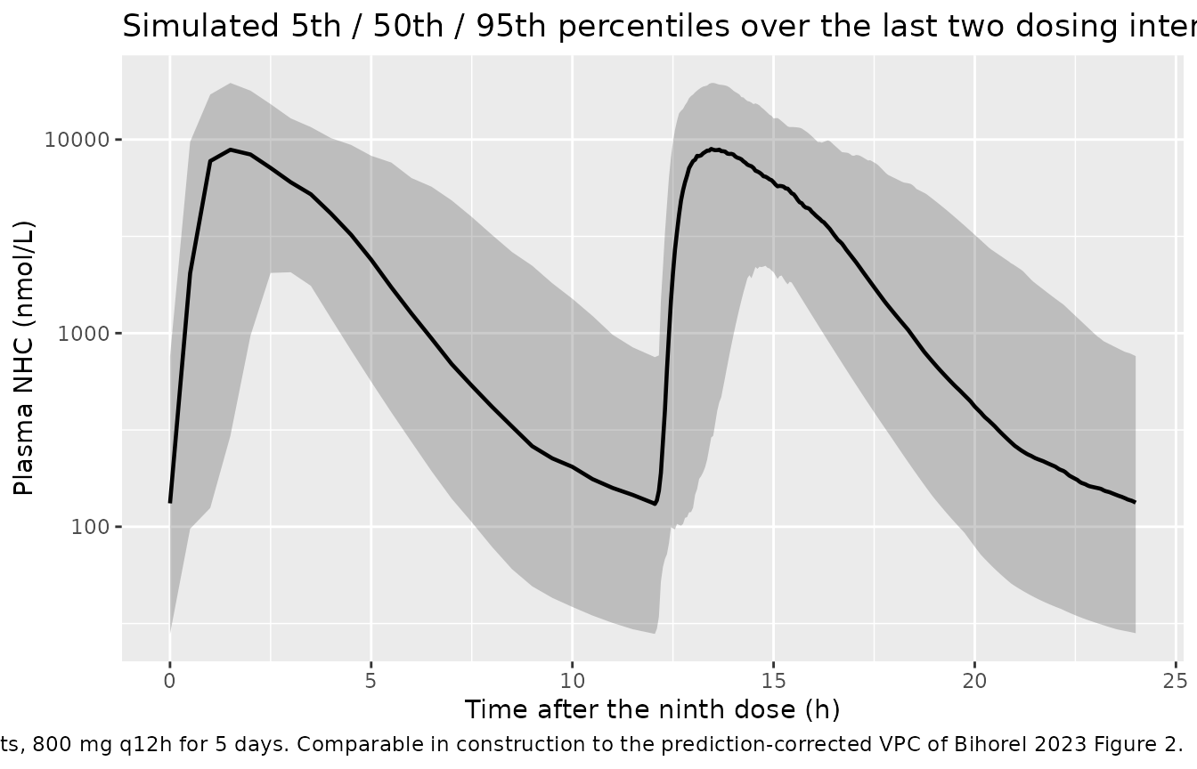
At steady state the model implies
AUC(0-12) = dose / (CL/F) exactly, which gives a
per-subject identity that does not depend on the drawn cohort.
auc_tau <- sim_cohort |>
  filter(time >= 108, !is.na(Cc)) |>
  group_by(id) |>
  arrange(time, .by_group = TRUE) |>
  summarise(
    auc12 = sum(diff(time) * (head(Cc, -1) + tail(Cc, -1)) / 2),
    WT = first(WT), .groups = "drop"
  ) |>
  # CL/F per subject, recovered from the identity AUC = dose / CL.
  mutate(cl_implied = DOSE_800MG_NMOL / auc12)

summary_tbl <- tibble(
  Quantity = c(
    "Median AUC(0-12) (nmol*h/L)",
    "5th percentile AUC(0-12)",
    "95th percentile AUC(0-12)",
    "Median CL/F implied by AUC (L/h)"
  ),
  Value = c(
    median(auc_tau$auc12), quantile(auc_tau$auc12, 0.05),
    quantile(auc_tau$auc12, 0.95), median(auc_tau$cl_implied)
  )
)
summary_tbl |>
  knitr::kable(digits = 0,
caption = "Simulated steady-state exposure, 800 mg q12h, 200 virtual participants.")| Quantity | Value |
|---|---|
| Median AUC(0-12) (nmol*h/L) | 33022 |
| 5th percentile AUC(0-12) | 17689 |
| 95th percentile AUC(0-12) | 70666 |
| Median CL/F implied by AUC (L/h) | 74 |
# Structural gates. These are centre / robust-quantile statements, not extremes,
# so they hold for any cohort this model can produce.
#  * The typical CL/F must sit near the published 70.6 L/h at 80 kg. The cohort
#    median weight is above 80 kg, so the median implied CL/F runs slightly high.
stopifnot(abs(median(auc_tau$cl_implied) - 70.6) / 70.6 < 0.25)
#  * The median AUC(0-12) must fall inside the paper's clinical comparability
#    bounds of 23,800-68,000 nmol*h/L (Methods).
stopifnot(median(auc_tau$auc12) > 23800, median(auc_tau$auc12) < 68000)
#  * AUC must fall with body weight (power -0.412 on CL/F). Compare the medians
#    of the lightest and heaviest weight terciles rather than any single subject.
terciles <- cut(auc_tau$WT, quantile(auc_tau$WT, c(0, 1/3, 2/3, 1)),
                include.lowest = TRUE, labels = c("light", "mid", "heavy"))
med_by_tercile <- tapply(auc_tau$auc12, terciles, median)
stopifnot(med_by_tercile[["light"]] > med_by_tercile[["heavy"]])
PKNCA validation
# Re-base time so the last dose sits at t = 0. `ev_typical` is a single
# deterministic subject, so rxSolve() returns no `id` column; PKNCA needs one,
# and adding it here is safe precisely because there is definitionally one
# subject in this arm.
sim_nca <- sim_typical |>
  filter(!is.na(Cc)) |>
  mutate(id = 1L, time = time - LAST_DOSE_TIME) |>
  filter(time >= 0) |>
  select(id, time, Cc, treatment)

# Guarantee a time-zero record per (id, treatment). Only `!is.na(Cc)` is used as
# a filter above, per the PKNCA recipe.
sim_nca <- bind_rows(
  sim_nca,
  sim_nca |> distinct(id, treatment) |> mutate(time = 0, Cc = 0)
) |>
  distinct(id, treatment, time, .keep_all = TRUE) |>
  arrange(id, treatment, time)

conc_obj <- PKNCA::PKNCAconc(sim_nca, Cc ~ time | treatment + id)

dose_df <- sim_nca |>
  distinct(id, treatment) |>
  mutate(time = 0, amt = DOSE_800MG_NMOL)
dose_obj <- PKNCA::PKNCAdose(dose_df, amt ~ time | treatment + id)

intervals <- data.frame(
  start     = c(0, 12),
  end       = c(12, Inf),
  cmax      = c(TRUE, FALSE),
  tmax      = c(TRUE, FALSE),
  auclast   = c(TRUE, FALSE),
  half.life = c(FALSE, TRUE)
)

nca_res <- PKNCA::pk.nca(PKNCA::PKNCAdata(conc_obj, dose_obj, intervals = intervals))
Comparison against published values
# PKNCA returns `tmax` for BOTH intervals, because it computes tmax internally
# as a dependency of half.life on the terminal interval -- and there the maximum
# sits at the interval start, giving tmax = 0. Averaging that with the real
# within-dose tmax of 1.5 h would report a spurious 0.75 h, so each parameter is
# taken from the interval it was actually requested on: peak and exposure from
# the 0-12 h dosing interval, half-life from the 12 h-onward terminal interval.
nca_long <- as.data.frame(nca_res$result) |>
  filter(
    (PPTESTCD %in% c("cmax", "tmax", "auclast") & start == 0) |
      (PPTESTCD == "half.life" & start == 12)
  ) |>
  select(treatment, PPTESTCD, PPORRES)

published <- tibble::tribble(
  ~treatment,             ~cmax, ~tmax, ~half.life, ~auclast,
  "Reference individual", 11400, 1.5,   16.5,       34000
)

cmp <- nlmixr2lib::ncaComparisonTable(
  simulated     = nca_long,
  reference     = published,
  by            = "treatment",
  units         = c(cmax = "nmol/L", tmax = "h", half.life = "h", auclast = "nmol*h/L"),
  tolerance_pct = 20
)

knitr::kable(
  cmp,
  caption = paste(
    "Simulated vs published typical values for the Bihorel 2023 reference",
    "individual (Discussion). * differs from the reference by >20%."
  )
)| NCA parameter | treatment | Reference | Simulated | % diff |
|---|---|---|---|---|
| Cmax (nmol/L) | Reference individual | 11400 | 11600 | +1.4% |
| Tmax (h) | Reference individual | 1.5 | 1.5 | +0.0% |
| AUClast (nmol*h/L) | Reference individual | 34000 | 34800 | +2.2% |
| t½ (h) | Reference individual | 16.5 | 16.5 | +0.1% |
The reference AUC(0-12) of 34,000 nmolh/L is not printed as such; it is recovered from the paper’s own printed correspondence in Methods, “the 0.7-2.0 range corresponds to plasma NHC AUC(0-12) of ~23,800-68,000 nmolh/L with molnupiravir 800 mg q12h”. Both endpoints invert to the same reference value (23,800 / 0.7 = 34,000 and 68,000 / 2.0 = 34,000), so the derivation is arithmetic on two printed numbers that agree, not a digitised or assumed value.
The simulated Cmax, Tmax, terminal half-life and AUC(0-12) all
reproduce the published typical values well within the 20% flagging
threshold, so the transcription of the absorption chain, the disposition
micro-constants and the molar dose conversion are all confirmed
simultaneously: an error in any one of them would move at least one of
the four. In particular Cmax and Tmax pin the absorption chain
(nn, mtt, ka), the half-life pins
the disposition micro-constants, and AUC(0-12) pins CL/F
together with the molar dose conversion.
Assumptions and deviations
-
Inter-occasion variability is implemented, with two
occasions. Bihorel 2023 places variability on the mean transit
time as IOV rather than IIV (Results, stage 3), and the Table 2 note
states that occasions were “labeled as occasion 1 and occasion 2” with
most participants having only one. The model therefore carries
etaiov_mtt_1andetaiov_mtt_2, the second fixed equal to the first to encode the shared NONMEM$OMEGA BLOCK(1) SAMEthat a single reported magnitude implies. Simulations here useOCC = 1throughout, which is the correct setting for every participant with COVID-19 and for the single-ascending-dose part of the phase I trial. -
Food status in the COVID-19 cohort is a modelling construct,
not data. Food status was not collected in any phase II or III
trial (Table 1). Bihorel 2023 assigned it by mixture modelling and,
after a sensitivity analysis, fixed at 25% the fraction of
unknown-food-status participants treated as having eaten a high-fat
meal; that assignment was then hard-coded into the analysis dataset. The
stochastic cohort above draws
FED_HIGHFAT ~ Bernoulli(0.25)to match. The paper’s own Limitations note that this assignment “may be confounded by disease status or other unknown covariates” and “could have impacted the estimation of other covariate effects”. - Body weight and BMI correlation is assumed. Table 1 reports both margins but not their joint distribution. The virtual cohort draws them from a bivariate normal with rho = 0.8, truncated to the reported ranges. Only the weight margin affects AUC (CL/F depends on weight alone), so the assumption influences the Cmax spread rather than the exposure gates above.
- Reduced variability structure for sparsely sampled participants is not reproduced. Bihorel 2023 estimated IIV only on CL/F for participants contributing fewer than three NHC measurements, because there were insufficient data to support two IIV terms and one IOV term (Results, stages 2 and 3). That is a per-record estimation device rather than a property of the final model, so the packaged model applies the full variability structure to every simulated subject. Simulated variability is therefore, if anything, slightly wider than the fitted model would produce for a sparse participant.
-
The hospitalisation effect on MTT is intentionally
absent. It was carried through stage 2 but was “close to 0 and
poorly estimated (RSE: 87.2%)” once the transit-compartment absorption
model was restored at stage 3, and it was the single relationship
removed by the final backward elimination. No final estimate is
published, so it cannot be encoded; see
covariatesDataExcluded. -
Screened-but-rejected covariates carry no
coefficients. Age, renal function, hepatic function, race and
ethnicity were all evaluated and none was retained. The paper reports
their effects only as forest-plot AUC(0-12) geometric mean ratios
(Figure 3), which are geometric means over shrunken empirical Bayes
estimates rather than typical-value contrasts and therefore cannot be
inverted into coefficients. They are documented in
covariatesDataExcludedand deliberately not gated on here. - No allometry on Q/F or Vp/F. This is the model as published; Bihorel 2023 Limitations flags the omission explicitly as the reason the model should not be extrapolated to children.
-
The analytical transit chain assumes one active
dose.
rxode2::transit()evaluates the Savic input rate from the most recent dose only. With a mean transit time of 0.435 h fasted and 2.27 h after a high-fat meal, the chain is effectively exhausted long before the next dose 12 h later, so superposition error is negligible at the regimens simulated here. It would not be for a regimen whose dosing interval approached the transit time. - No parameter value came from anywhere other than the paper’s own text and tables. No figure digitisation, no author correspondence and no upstream model were needed; Table 2 reports the complete final parameter set. The supplement (Tables S1-S3, Figures S1-S10) holds sampling schedules, the modified Child-Pugh criteria, sample-exclusion accounting and diagnostic plots, none of which carry a model parameter. A Crossref check found no erratum or correction notice for doi:10.1002/psp4.13031.