Mycophenolic acid (Park 2023)
Source:vignettes/articles/Park_2023_mycophenolic_acid.Rmd
Park_2023_mycophenolic_acid.RmdModel and source
- Citation: Park HJ, Hong KT, Han N, Kim I-W, Oh JM, Kang HJ. Body Surface Area-Based Dosing of Mycophenolate Mofetil in Pediatric Hematopoietic Stem Cell Transplant Recipients: A Prospective Population Pharmacokinetic Study. Pharmaceutics. 2023;15(12):2741. doi:10.3390/pharmaceutics15122741.
- Description: Population PK model for total mycophenolic acid (MPA, the active moiety of mycophenolate mofetil MMF) in pediatric allogeneic haematopoietic stem cell transplantation (HSCT) recipients receiving oral MMF for acute graft-versus-host disease prophylaxis or treatment (Park 2023). One-compartment disposition with first-order absorption and no lag time (NONMEM ADVAN2 TRANS2). Body surface area is the only retained covariate, entering the apparent volume of distribution as a centered-linear term Vd/F = 89.83 * (1 + 0.854 * (BSA - 1.11)). Inter-individual variability is log-normal on CL/F and Vd/F; residual error is combined proportional plus additive. Doses are MMF mass (mg) with no MMF-to-MPA molecular-weight conversion – CL/F and Vd/F are apparent parameters that absorb both the molecular-weight ratio and oral bioavailability.
- Article: https://doi.org/10.3390/pharmaceutics15122741
Park 2023 is a prospective single-centre population pharmacokinetic study of oral mycophenolate mofetil (MMF) in paediatric allogeneic haematopoietic stem cell transplantation (HSCT) recipients. Total mycophenolic acid (MPA) — the active moiety — was described by a one-compartment model with first-order absorption (NONMEM ADVAN2 TRANS2). Body surface area (BSA) was the single retained covariate and acts on the apparent volume of distribution.
Population
Twenty paediatric HSCT recipients contributed 80 total MPA serum concentrations (Park 2023 Table 1). Median age was 9.7 years (range 1.7–15.6); 14 patients (70%) were 1 to under 12 years old and 6 (30%) were 12 to under 18. Twelve patients (60%) were male. Median body weight was 31.2 kg (9.9–51.0), median height 136.0 cm (83.6–176.9), and median BSA 1.12 m^2 (0.49–1.60). Race and ethnicity are not tabulated; the study was conducted at Seoul National University Hospital.
Underlying diagnoses were acute lymphoblastic leukaemia (7), acute myeloid leukaemia (5), aplastic anaemia (2), non-Hodgkin lymphoma (2), and one each of congenital neutropenia, haemophagocytic lymphohistiocytosis, Krabbe disease, and therapy-related myelodysplastic syndrome. Sixteen patients (80%) received a haploidentical family graft. All 20 had previous or concomitant tacrolimus. MMF was started for aGVHD prophylaxis in 16 patients (80%) and for treatment in 4 (20%); 11 patients (55%) went on to develop aGVHD, 4 with grade III–IV.
Renal and hepatic function were essentially normal — median serum creatinine 0.42 mg/dL, median eGFR 112.6 mL/min/1.73 m^2, median total bilirubin 0.5 mg/dL, median albumin 3.8 g/dL — which the authors cite as the reason that renal- and hepatic-function covariates retained in solid-organ transplant models were not significant here.
Oral MMF was given at 15–20 mg/kg twice daily (median 17.9 mg/kg/dose, range 16.1–19.8; median 1100 mg/day, range 380–2000) as capsule (30%) or oral suspension (70%). Sampling followed a limited-sampling strategy at pre-dose and 1, 2 and 6 h post-dose, drawn at least 3 days after MMF initiation so that MPA was at steady state. Total MPA was assayed by PETINIA with an LLOQ of 0.1 mg/L.
The same information is available programmatically via the model’s
population metadata
(readModelDb("Park_2023_mycophenolic_acid")()$population).
Source trace
The per-parameter origin is recorded as an in-file comment next to
each ini() entry in
inst/modeldb/specificDrugs/Park_2023_mycophenolic_acid.R.
The table below collects them in one place for review.
| Equation / parameter | Value | Source location |
|---|---|---|
lka (ka) |
5.18 1/h | Table 4, “Final Model” column, row ka (RSE 21%) |
lvc (Vd/F) |
89.83 L | Equation 2 (Table 4 rounds the same estimate to 89.8 L, RSE 16%) |
lcl (CL/F) |
16.6 L/h | Table 4, “Final Model” column, row CL/F (RSE 17%) |
e_bsa_vc |
0.854 per m^2 | Table 4, “Final Model” column, row BSA on Vd/F (RSE
24%); Equation 2 prints it rounded to 0.85 |
| BSA centering value | 1.11 m^2 | Text immediately below Equation 2 (“where 1.11 m^2 was the median value of BSA”) |
etalvc |
omega^2 = 0.13296 | Table 4 IIV Vd/F 37.71 %CV, inverted through the Table 4 footnote
%CV = sqrt(exp(OMEGA) - 1) * 100
|
etalcl |
omega^2 = 0.59293 | Table 4 IIV CL/F 89.96 %CV, inverted through the same footnote |
propSd |
0.660 | Table 4, row Proportional error (RSE 9%); read as an SD
— see Errata |
addSd |
0.111 | Table 4, row Additive error (RSE 17%); read as an SD —
see Errata |
| One-compartment, first-order absorption, no lag | n/a | Results 3.2.2 (“A one-compartment model with first-order absorption (ADVAN2 TRANS2 subroutine) was selected”) |
Exponential IIV Pi = theta * exp(eta_Pi)
|
n/a | Equation 1 |
| Combined proportional + additive residual error | n/a | Results 3.2.2 (“A combined residual error model was selected”) |
Vd/F = 89.83 * (1 + 0.854 * (BSA - 1.11)) |
n/a | Equation 2 |
The Table 4 footnote is what removes the usual CV%-versus-omega
ambiguity for the IIV terms: because Park 2023 states
%CV = sqrt(exp(OMEGA) - 1) * 100 explicitly, the tabulated
percentages are exact log-normal CVs and OMEGA is
unambiguously the variance of eta. No approximation is needed.
Virtual cohort
Original observed data are not publicly available. The cohort below is deterministic: 200 subjects are placed at evenly spaced quantiles and each body-size variable is piecewise-linearly interpolated between the median and range that Park 2023 Table 1 reports. This reproduces the published median and range exactly by construction, keeps weight / height / BSA mutually monotone (as they are in a paediatric cohort), and avoids the sampling noise that a random draw of 200 would introduce into the validation comparison.
set.seed(20231207)

n_sub <- 200L

# Piecewise-linear interpolation of a (min, median, max) triple onto evenly
# spaced quantiles. Table 1 of Park 2023 reports exactly this triple for
# weight, height and BSA.
interp_triple <- function(p, lo, mid, hi) {
  ifelse(p <= 0.5, lo + (mid - lo) * (p / 0.5), mid + (hi - mid) * ((p - 0.5) / 0.5))
}

p_grid <- (seq_len(n_sub) - 0.5) / n_sub

cohort <- tibble(
  id  = seq_len(n_sub),
  WT  = interp_triple(p_grid,  9.9,  31.2,  51.0),   # Park 2023 Table 1
  HT  = interp_triple(p_grid, 83.6, 136.0, 176.9),   # Park 2023 Table 1
  BSA = interp_triple(p_grid, 0.49,  1.12,   1.60)   # Park 2023 Table 1
) |>
  # Median 17.9 mg/kg/dose (Park 2023 Table 1) applied to every subject.
  mutate(amt_mg = 17.9 * WT)

# Confirm the cohort reproduces the published summary statistics.
tibble(
  Statistic = c("Weight (kg)", "Height (cm)", "BSA (m^2)", "Dose (mg/dose)"),
  Published = c("31.2 (9.9-51.0)", "136.0 (83.6-176.9)", "1.12 (0.49-1.60)",
                "550 (190-1000)"),
  Simulated = c(
    sprintf("%.1f (%.1f-%.1f)", median(cohort$WT),  min(cohort$WT),  max(cohort$WT)),
    sprintf("%.1f (%.1f-%.1f)", median(cohort$HT),  min(cohort$HT),  max(cohort$HT)),
    sprintf("%.2f (%.2f-%.2f)", median(cohort$BSA), min(cohort$BSA), max(cohort$BSA)),
    sprintf("%.0f (%.0f-%.0f)", median(cohort$amt_mg), min(cohort$amt_mg), max(cohort$amt_mg))
  )
) |>
knitr::kable(caption = "Virtual cohort versus Park 2023 Table 1, median (range).")| Statistic | Published | Simulated |
|---|---|---|
| Weight (kg) | 31.2 (9.9-51.0) | 31.2 (10.0-50.9) |
| Height (cm) | 136.0 (83.6-176.9) | 136.0 (83.9-176.7) |
| BSA (m^2) | 1.12 (0.49-1.60) | 1.12 (0.49-1.60) |
| Dose (mg/dose) | 550 (190-1000) | 558 (179-911) |
Dosing is twice daily at steady state (ss = 1,
ii = 12), matching the study design: samples were drawn at
least three days after MMF initiation specifically “to ensure that the
MPA concentration had reached a steady-state concentration”.
Observations are placed on the central ODE state;
rxode2 returns the algebraic observable Cc as
a column at those rows.
obs_times <- sort(unique(c(seq(0, 12, by = 0.1), c(0, 1, 2, 6))))

dose_rows <- cohort |>
  transmute(id, time = 0, amt = amt_mg, evid = 1L, ii = 12, ss = 1L,
            cmt = "depot", BSA, WT)

obs_rows <- cohort |>
  select(id, BSA, WT) |>
  crossing(time = obs_times) |>
  transmute(id, time, amt = NA_real_, evid = 0L, ii = 0, ss = 0L,
            cmt = "central", BSA, WT)

events <- bind_rows(dose_rows, obs_rows) |>
  arrange(id, time, desc(evid))

stopifnot(!anyDuplicated(unique(events[, c("id", "time", "evid")])))
Simulation
mod <- readModelDb("Park_2023_mycophenolic_acid")

# Population simulation: between-subject variability on.
#
# rxode2 returns three concentration columns. `Cc` is the individual
# prediction (IPRED) -- it carries IIV but NOT residual error -- while `sim`
# is the simulated observation, IPRED plus the combined proportional and
# additive residual error. The published Table 2 NCA was computed from
# measured concentrations, so `sim` is the like-for-like column and `Cc` is
# not. Negative draws (possible because the error model has an additive
# term) are floored at zero, as a real assay would report them.
# steady-state searches for long-half-life subjects exceed the default step budget
sim_pop <- rxode2::rxSolve(mod, events = events, keep = c("BSA", "WT"),
                           maxsteps = 1e6) |>
  as.data.frame() |>
  mutate(Cobs = pmax(sim, 0))
#> ℹ parameter labels from comments will be replaced by 'label()'

# Typical-value simulation: `omega = NA` / `sigma = NA` suppress IIV and
# residual error for this call only. (`zeroRe()` mutates shared model state
# and is deliberately avoided.) Here `Cc` is the typical-value prediction.
sim_typ <- rxode2::rxSolve(mod, events = events, keep = c("BSA", "WT"),
                           omega = NA, sigma = NA,
                           # steady-state searches for long-half-life subjects exceed the default step budget
                           maxsteps = 1e6) |>
  as.data.frame() |>
  mutate(Cobs = Cc)

nrow(sim_pop)
#> [1] 24200
Replicate published figures
Figure 1 — MPA concentration-time profiles
Park 2023 Figure 1 plots the individual observed MPA concentrations over the 0–6 h sampling window with the mean profile overlaid. The simulated equivalent below shows the typical-value profile and the 5th–95th percentile band of the virtual cohort.
# Replicates Figure 1 of Park 2023: MPA plasma concentration-time profiles.
# Percentiles are taken on the observation scale (`Cobs` = IPRED + residual
# error), matching the individual measured concentrations plotted in the
# published figure.
prof <- sim_pop |>
  filter(time <= 6) |>
  group_by(time) |>
  summarise(Q05 = quantile(Cobs, 0.05), Q50 = quantile(Cobs, 0.50),
            Q95 = quantile(Cobs, 0.95), .groups = "drop")

typ <- sim_typ |> filter(time <= 6) |> group_by(time) |>
  summarise(Cc = median(Cc), .groups = "drop")

ggplot(prof, aes(time, Q50)) +
  geom_ribbon(aes(ymin = Q05, ymax = Q95), alpha = 0.2, fill = "steelblue") +
  geom_line(colour = "steelblue", linewidth = 0.9) +
  geom_line(data = typ, aes(time, Cc), colour = "firebrick",
            linetype = "dashed", linewidth = 0.9) +
  scale_x_continuous(breaks = c(0, 1, 2, 4, 6)) +
  labs(x = "Time after dose (h)", y = "MPA concentration (mg/L)",
       title = "Figure 1 - simulated MPA concentration-time profile",
       subtitle = paste("Blue: virtual-cohort median with 5th-95th percentile band.",
                        "Red dashed: typical value."),
       caption = "Replicates Figure 1 of Park 2023.")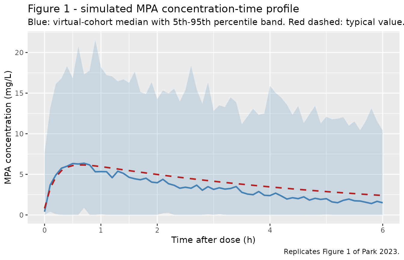
The observed data in Park 2023 Figure 1 peak at the 1 h sampling point and decline to roughly 1 mg/L by 6 h, which the simulated profile reproduces. Note that the model’s true peak occurs earlier than the first post-dose sample:
ka  <- 5.18
kel <- 16.6 / (89.83 * (1 + 0.854 * (1.12 - 1.11)))
tmax_true <- log(ka / kel) / (ka - kel)
sprintf("Model true Tmax = %.2f h; earliest post-dose sample in the study = 1 h", tmax_true)
#> [1] "Model true Tmax = 0.67 h; earliest post-dose sample in the study = 1 h"
The limited-sampling design therefore cannot observe the true peak; the reported Tmax of 1 h is the first sampling time, not an estimate of the peak time. This matters for the Cmax comparison below.
Figure 5 — simulated AUC0-12 by BSA and dose
Park 2023 Figure 5 simulates AUC0-12 at BSA of 0.5, 1.0 and 1.5 m^2 under 400, 600 and 900 mg/m^2 twice-daily dosing, and concludes that 900 mg/m^2 BID is the regimen that lands within the 30–60 mg*h/L therapeutic target.
fig5_grid <- expand_grid(
  dose_per_m2 = c(400, 600, 900),
  BSA         = c(0.5, 1.0, 1.5)
) |>
  mutate(arm = sprintf("%d mg/m^2, BSA %.1f", dose_per_m2, BSA),
         arm_id = row_number())

n_arm <- 200L

fig5_subj <- fig5_grid |>
  rowwise() |>
  reframe(
    arm, dose_per_m2, BSA,
    id = (arm_id - 1L) * n_arm + seq_len(n_arm),
    amt_mg = dose_per_m2 * BSA
  )

# Disjoint ids across arms are mandatory - rxSolve keys on id alone.
stopifnot(!anyDuplicated(fig5_subj$id))

f5_obs_times <- seq(0, 12, by = 0.25)

f5_events <- bind_rows(
  fig5_subj |>
    transmute(id, time = 0, amt = amt_mg, evid = 1L, ii = 12, ss = 1L,
              cmt = "depot", BSA, arm),
  fig5_subj |>
    select(id, BSA, arm) |>
    crossing(time = f5_obs_times) |>
    transmute(id, time, amt = NA_real_, evid = 0L, ii = 0, ss = 0L,
              cmt = "central", BSA, arm)
) |>
  arrange(id, time, desc(evid))

# steady-state searches for long-half-life subjects exceed the default step budget
f5_sim <- rxode2::rxSolve(mod, events = f5_events, keep = c("BSA", "arm"),
                          maxsteps = 1e6) |>
  as.data.frame()

# Deterministic companion run: one subject per arm, no IIV, on a fine grid.
# The steady-state identity AUC0-tau = Dose/(CL/F) is a structural property,
# so it is checked here rather than against the population median, whose
# sampling error at n = 200 with an 89.96 %CV IIV on CL/F is about 7% --
# far too noisy to gate a 1% structural assertion.
f5_typ_events <- bind_rows(
  fig5_grid |>
    transmute(id = arm_id, time = 0, amt = dose_per_m2 * BSA, evid = 1L,
              ii = 12, ss = 1L, cmt = "depot", BSA, arm),
  fig5_grid |>
    select(arm_id, BSA, arm) |>
    crossing(time = seq(0, 12, by = 0.05)) |>
    transmute(id = arm_id, time, amt = NA_real_, evid = 0L, ii = 0, ss = 0L,
              cmt = "central", BSA, arm)
) |>
  arrange(id, time, desc(evid))

f5_typ_auc <- rxode2::rxSolve(mod, events = f5_typ_events, keep = c("BSA", "arm"),
                              omega = NA, sigma = NA,
                              # steady-state searches for long-half-life subjects exceed the default step budget
                              maxsteps = 1e6) |>
  as.data.frame() |>
  arrange(id, time) |>
  group_by(arm) |>
  summarise(auc12_typ = sum(diff(time) * (head(Cc, -1) + tail(Cc, -1)) / 2),
            .groups = "drop")
# Replicates Figure 5 of Park 2023: simulated AUC0-12 by BSA and dose level.
f5_auc <- f5_sim |>
  arrange(id, time) |>
  group_by(id, arm) |>
  summarise(
    auc12 = sum(diff(time) * (head(Cc, -1) + tail(Cc, -1)) / 2),
    .groups = "drop"
  ) |>
  mutate(
    dose_per_m2 = as.integer(sub(" mg.*", "", arm)),
    BSA = as.numeric(sub(".*BSA ", "", arm))
  )

ggplot(f5_auc, aes(factor(BSA), auc12)) +
  geom_boxplot(outlier.size = 0.4, fill = "steelblue", alpha = 0.5) +
  geom_hline(yintercept = c(30, 60), colour = "firebrick") +
  facet_wrap(~ paste0("Dose ", dose_per_m2, " mg/m^2")) +
  coord_cartesian(ylim = c(0, 200)) +
  labs(x = expression(BSA~(m^2)), y = "AUC0-12 (mg*h/L)",
       title = "Figure 5 - simulated AUC0-12 with different dosing regimens",
       caption = "Replicates Figure 5 of Park 2023. Red lines: 30-60 mg*h/L target.")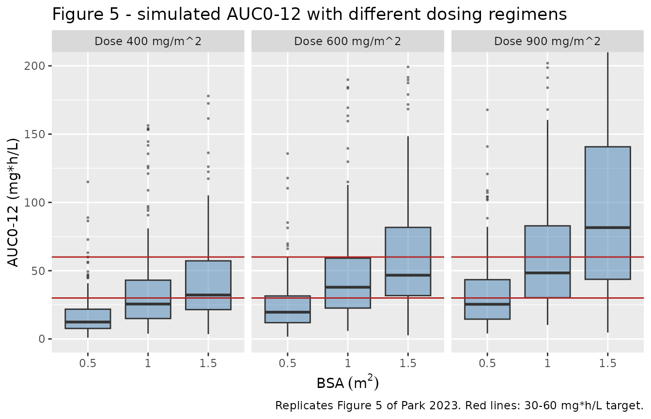
The simulated distribution does not match the
published Figure 5. The comparison below digitises the published box
medians and puts them alongside both the simulation and the exact
steady-state identity AUC0-tau,ss = Dose / (CL/F), which
any linear one-compartment model must satisfy regardless of absorption
rate or volume.
published_fig5 <- tibble::tribble(
  ~dose_per_m2, ~BSA, ~fig5_median,
  400L, 0.5, 16.7,  400L, 1.0, 17.2,  400L, 1.5, 17.9,
  600L, 0.5, 22.3,  600L, 1.0, 22.7,  600L, 1.5, 23.0,
  900L, 0.5, 30.3,  900L, 1.0, 30.6,  900L, 1.5, 31.2
)

fig5_compare <- f5_auc |>
  group_by(arm, dose_per_m2, BSA) |>
  summarise(sim_median = median(auc12), .groups = "drop") |>
  left_join(f5_typ_auc, by = "arm") |>
  left_join(published_fig5, by = c("dose_per_m2", "BSA")) |>
  mutate(
    identity_dose_over_cl = dose_per_m2 * BSA / 16.6,
    ratio_typ_vs_fig5     = auc12_typ / fig5_median
  ) |>
  arrange(dose_per_m2, BSA)

fig5_compare |>
  select(-arm) |>
  rename(
    "Dose (mg/m^2)"               = dose_per_m2,
    "BSA (m^2)"                   = BSA,
    "Cohort median"               = sim_median,
    "Typical value"               = auc12_typ,
    "Figure 5 median (digitised)" = fig5_median,
    "Dose/(CL/F) identity"        = identity_dose_over_cl,
    "Typical / Figure 5"          = ratio_typ_vs_fig5
  ) |>
  knitr::kable(digits = 2,
               caption = paste("Simulated AUC0-12 versus the digitised Park 2023",
                               "Figure 5. The typical-value column is",
                               "deterministic; the cohort median carries about",
"7% sampling error at n = 200."))| Dose (mg/m^2) | BSA (m^2) | Cohort median | Typical value | Figure 5 median (digitised) | Dose/(CL/F) identity | Typical / Figure 5 |
|---|---|---|---|---|---|---|
| 400 | 0.5 | 11.71 | 12.04 | 16.7 | 12.05 | 0.72 |
| 400 | 1.0 | 23.37 | 24.09 | 17.2 | 24.10 | 1.40 |
| 400 | 1.5 | 34.56 | 36.14 | 17.9 | 36.14 | 2.02 |
| 600 | 0.5 | 17.74 | 18.06 | 22.3 | 18.07 | 0.81 |
| 600 | 1.0 | 37.28 | 36.14 | 22.7 | 36.14 | 1.59 |
| 600 | 1.5 | 54.42 | 54.21 | 23.0 | 54.22 | 2.36 |
| 900 | 0.5 | 23.08 | 27.10 | 30.3 | 27.11 | 0.89 |
| 900 | 1.0 | 53.01 | 54.20 | 30.6 | 54.22 | 1.77 |
| 900 | 1.5 | 88.42 | 81.31 | 31.2 | 81.33 | 2.61 |
Three independent features of Figure 5 are inconsistent with the model parameters printed in Table 4 and Equation 2 of the same paper:
-
Level. At 900 mg/m^2 and BSA 1.0 m^2 the dose is
900 mg and the steady-state identity gives
900 / 16.6 = 54.2 mg*h/L. The published box median is about 30.6. -
Dose proportionality. A linear model forces AUC to
be strictly proportional to dose. The published medians at BSA 1.0 m^2
are 17.2, 22.7 and 30.6 for doses in the ratio 1 : 1.5 : 2.25 — ratios
of 1 : 1.32 : 1.78. They are instead fit almost exactly by
AUC = 4.2 + 0.030 * dose, and a non-zero intercept is not attainable from any linear one-compartment model. -
BSA independence. The published medians are nearly
flat across BSA within each dose panel (30.3, 30.6, 31.2 at 900 mg/m^2).
That is what a fixed mg dose would produce, because
CL/Fcarries no covariate — but it contradicts the mg/m^2 dose labels, under which a threefold BSA change must produce a threefold AUC change.
Feature 3 alone could be explained by the simulation having used fixed mg doses despite the mg/m^2 labels, but features 1 and 2 survive that reading as well. Figure 5 is therefore not reproducible from the published parameters; see Errata. The model file encodes Table 4 and Equation 2, which are internally consistent and, as the next section shows, reproduce the paper’s own non-compartmental results.
PKNCA validation
Park 2023 Table 2 reports non-compartmental parameters computed from
the observed limited-sampling profiles (pre-dose, 1, 2 and 6 h). The NCA
below mirrors that design exactly: it uses only those
four sampling times, and — as the paper did — treats the steady-state
profile as if it were a single dose so that AUC0-inf and
CL/F = Dose / AUC0-inf are defined.
nca_times <- c(0, 1, 2, 6)

make_nca <- function(sim, label) {
  conc <- sim |>
    filter(!is.na(Cobs), time %in% nca_times) |>
    transmute(id, time, Cc = Cobs, scale = label)

  dose <- cohort |>
    transmute(id, time = 0, amt = amt_mg, scale = label)

  conc_obj <- PKNCA::PKNCAconc(as.data.frame(conc), Cc ~ time | scale + id)
  dose_obj <- PKNCA::PKNCAdose(as.data.frame(dose), amt ~ time | scale + id)

  intervals <- data.frame(
    start = 0, end = c(6, Inf),
    cmax = c(TRUE, FALSE), tmax = c(TRUE, FALSE),
    auclast = c(TRUE, FALSE),
    aucinf.obs = c(FALSE, TRUE), half.life = c(FALSE, TRUE),
    cl.obs = c(FALSE, TRUE), vz.obs = c(FALSE, TRUE)
  )

  # The limited-sampling design leaves only three post-dose points (1, 2 and
  # 6 h). PKNCA excludes Tmax from the terminal-slope fit by default, which
  # would leave two points and fail the three-point minimum, so lambda_z is
  # allowed to use the Tmax point here. The paper's own NCA (PK Solver /
  # NonCompart) necessarily did the same to report AUC0-inf from these data.
  PKNCA::pk.nca(PKNCA::PKNCAdata(
    conc_obj, dose_obj, intervals = intervals,
    options = list(allow.tmax.in.half.life = TRUE)
  ))
}

nca_pop <- make_nca(sim_pop, "Virtual cohort (IIV + residual error)")
#> Warning: Too few points for half-life calculation (min.hl.points=3 with only 2 points)
#> Too few points for half-life calculation (min.hl.points=3 with only 2 points)
#> Too few points for half-life calculation (min.hl.points=3 with only 2 points)
#> Warning: Too few points for half-life calculation (min.hl.points=3 with only 1 points)
#> Too few points for half-life calculation (min.hl.points=3 with only 1 points)
#> Warning: Too few points for half-life calculation (min.hl.points=3 with only 2
#> points)
#> Warning: Too few points for half-life calculation (min.hl.points=3 with only 1
#> points)
#> Warning: Too few points for half-life calculation (min.hl.points=3 with only 2 points)
#> Too few points for half-life calculation (min.hl.points=3 with only 2 points)
#> Too few points for half-life calculation (min.hl.points=3 with only 2 points)
#> Too few points for half-life calculation (min.hl.points=3 with only 2 points)
#> Too few points for half-life calculation (min.hl.points=3 with only 2 points)
#> Too few points for half-life calculation (min.hl.points=3 with only 2 points)
#> Too few points for half-life calculation (min.hl.points=3 with only 2 points)
#> Too few points for half-life calculation (min.hl.points=3 with only 2 points)
#> Too few points for half-life calculation (min.hl.points=3 with only 2 points)
#> Too few points for half-life calculation (min.hl.points=3 with only 2 points)
#> Too few points for half-life calculation (min.hl.points=3 with only 2 points)
#> Warning: Too few points for half-life calculation (min.hl.points=3 with only 1
#> points)
#> Warning: Too few points for half-life calculation (min.hl.points=3 with only 2 points)
#> Too few points for half-life calculation (min.hl.points=3 with only 2 points)
#> Too few points for half-life calculation (min.hl.points=3 with only 2 points)
#> Too few points for half-life calculation (min.hl.points=3 with only 2 points)
#> Too few points for half-life calculation (min.hl.points=3 with only 2 points)
#> Too few points for half-life calculation (min.hl.points=3 with only 2 points)
#> Too few points for half-life calculation (min.hl.points=3 with only 2 points)
#> Warning: Too few points for half-life calculation (min.hl.points=3 with only 1
#> points)
#> Warning: Too few points for half-life calculation (min.hl.points=3 with only 2
#> points)
#> Warning: Too few points for half-life calculation (min.hl.points=3 with only 1
#> points)
#> Warning: Too few points for half-life calculation (min.hl.points=3 with only 2
#> points)
#> Warning: Too few points for half-life calculation (min.hl.points=3 with only 1
#> points)
#> Warning: Too few points for half-life calculation (min.hl.points=3 with only 2 points)
#> Too few points for half-life calculation (min.hl.points=3 with only 2 points)
#> Warning: Too few points for half-life calculation (min.hl.points=3 with only 1 points)
#> Too few points for half-life calculation (min.hl.points=3 with only 1 points)
#> Warning: Too few points for half-life calculation (min.hl.points=3 with only 2 points)
#> Too few points for half-life calculation (min.hl.points=3 with only 2 points)
#> Too few points for half-life calculation (min.hl.points=3 with only 2 points)
#> Too few points for half-life calculation (min.hl.points=3 with only 2 points)
#> Too few points for half-life calculation (min.hl.points=3 with only 2 points)
#> Too few points for half-life calculation (min.hl.points=3 with only 2 points)
#> Warning: Too few points for half-life calculation (min.hl.points=3 with only 1
#> points)
#> Warning: Too few points for half-life calculation (min.hl.points=3 with only 2 points)
#> Too few points for half-life calculation (min.hl.points=3 with only 2 points)
#> Too few points for half-life calculation (min.hl.points=3 with only 2 points)
#> Warning: Too few points for half-life calculation (min.hl.points=3 with only 1
#> points)
#> Warning: Too few points for half-life calculation (min.hl.points=3 with only 2 points)
#> Too few points for half-life calculation (min.hl.points=3 with only 2 points)
#> Too few points for half-life calculation (min.hl.points=3 with only 2 points)
#> Too few points for half-life calculation (min.hl.points=3 with only 2 points)
#> Too few points for half-life calculation (min.hl.points=3 with only 2 points)
#> Too few points for half-life calculation (min.hl.points=3 with only 2 points)
#> Too few points for half-life calculation (min.hl.points=3 with only 2 points)
#> Too few points for half-life calculation (min.hl.points=3 with only 2 points)
#> Too few points for half-life calculation (min.hl.points=3 with only 2 points)
#> Warning: Too few points for half-life calculation (min.hl.points=3 with only 1
#> points)
#> Warning: Too few points for half-life calculation (min.hl.points=3 with only 2 points)
#> Too few points for half-life calculation (min.hl.points=3 with only 2 points)
#> Too few points for half-life calculation (min.hl.points=3 with only 2 points)
#> Too few points for half-life calculation (min.hl.points=3 with only 2 points)
#> Too few points for half-life calculation (min.hl.points=3 with only 2 points)
#> Too few points for half-life calculation (min.hl.points=3 with only 2 points)
#> Warning: Too few points for half-life calculation (min.hl.points=3 with only 1
#> points)
#> Warning: Too few points for half-life calculation (min.hl.points=3 with only 2 points)
#> Too few points for half-life calculation (min.hl.points=3 with only 2 points)
#> Too few points for half-life calculation (min.hl.points=3 with only 2 points)
#> Too few points for half-life calculation (min.hl.points=3 with only 2 points)
#> Warning: Too few points for half-life calculation (min.hl.points=3 with only 1
#> points)
#> Warning: Too few points for half-life calculation (min.hl.points=3 with only 2 points)
#> Too few points for half-life calculation (min.hl.points=3 with only 2 points)
#> Too few points for half-life calculation (min.hl.points=3 with only 2 points)
#> Too few points for half-life calculation (min.hl.points=3 with only 2 points)
#> Warning: Too few points for half-life calculation (min.hl.points=3 with only 1
#> points)
#> Warning: Too few points for half-life calculation (min.hl.points=3 with only 2 points)
#> Too few points for half-life calculation (min.hl.points=3 with only 2 points)
#> Too few points for half-life calculation (min.hl.points=3 with only 2 points)
#> Warning: Too few points for half-life calculation (min.hl.points=3 with only 1 points)
#> Too few points for half-life calculation (min.hl.points=3 with only 1 points)
#> Warning: Too few points for half-life calculation (min.hl.points=3 with only 2 points)
#> Too few points for half-life calculation (min.hl.points=3 with only 2 points)
#> Too few points for half-life calculation (min.hl.points=3 with only 2 points)
#> Too few points for half-life calculation (min.hl.points=3 with only 2 points)
#> Warning: Too few points for half-life calculation (min.hl.points=3 with only 1 points)
#> Too few points for half-life calculation (min.hl.points=3 with only 1 points)
#> Warning: Too few points for half-life calculation (min.hl.points=3 with only 2 points)
#> Too few points for half-life calculation (min.hl.points=3 with only 2 points)
#> Too few points for half-life calculation (min.hl.points=3 with only 2 points)
#> Too few points for half-life calculation (min.hl.points=3 with only 2 points)
#> Warning: Too few points for half-life calculation (min.hl.points=3 with only 1
#> points)
#> Warning: Too few points for half-life calculation (min.hl.points=3 with only 2
#> points)
#> Warning: Too few points for half-life calculation (min.hl.points=3 with only 1
#> points)
#> Warning: Too few points for half-life calculation (min.hl.points=3 with only 2 points)
#> Too few points for half-life calculation (min.hl.points=3 with only 2 points)
#> Too few points for half-life calculation (min.hl.points=3 with only 2 points)
#> Warning: Too few points for half-life calculation (min.hl.points=3 with only 1 points)
#> Too few points for half-life calculation (min.hl.points=3 with only 1 points)
#> Warning: Too few points for half-life calculation (min.hl.points=3 with only 2 points)
#> Too few points for half-life calculation (min.hl.points=3 with only 2 points)
#> Too few points for half-life calculation (min.hl.points=3 with only 2 points)
#> Warning: Too few points for half-life calculation (min.hl.points=3 with only 1
#> points)
#> Warning: Too few points for half-life calculation (min.hl.points=3 with only 2 points)
#> Too few points for half-life calculation (min.hl.points=3 with only 2 points)
#> Too few points for half-life calculation (min.hl.points=3 with only 2 points)
#> Warning: Too few points for half-life calculation (min.hl.points=3 with only 1
#> points)
#> Warning: Too few points for half-life calculation (min.hl.points=3 with only 2 points)
#> Too few points for half-life calculation (min.hl.points=3 with only 2 points)
nca_typ <- make_nca(sim_typ, "Typical value (no IIV, no residual error)")
Comparison against published NCA
Park 2023 Table 2 reports arithmetic means. PKNCA’s
own summary method aggregates by median, so the per-subject results are
aggregated here with mean() to compare like with like. Two
scales are reported in the same table: the typical-value prediction and
the full virtual-cohort population mean. This matters because the
model’s IIV on CL/F is large (89.96 %CV), so for a log-normal parameter
the population mean exposure sits roughly
exp(omega^2 / 2) = 1.34-fold above the
typical (median) exposure.
half.life is computed but has no published counterpart —
Park 2023 Table 2 does not report a terminal half-life — so it is shown
separately below rather than in the comparison table.
summarise_nca <- function(res, label) {
  as.data.frame(res) |>
    filter(!is.na(PPORRES)) |>
    # PKNCA emits dependency rows; keep only the requested interval endpoints.
    filter((PPTESTCD %in% c("cmax", "tmax", "auclast") & end == 6) |
           (PPTESTCD %in% c("aucinf.obs", "half.life", "cl.obs", "vz.obs") & is.infinite(end))) |>
    group_by(PPTESTCD) |>
    summarise(value = mean(PPORRES), .groups = "drop") |>
    pivot_wider(names_from = PPTESTCD, values_from = value) |>
    mutate(scale = label)
}

simulated_nca <- bind_rows(
  summarise_nca(nca_typ, "Typical value (no IIV, no residual error)"),
  summarise_nca(nca_pop, "Virtual cohort (IIV + residual error)")
)

# Park 2023 Table 2, mean values (n = 20).
#
# Tmax needs a different reference per scale, because the paper reports two
# different things. Results 3.2 states "The tmax was at 1 h after the MMF
# administration" -- that is where the peak sample sits, and it is the
# right comparator for the noise-free typical-value run. Table 3 reports the
# arithmetic mean of the observed per-subject Tmax (1.29 h in the 7 aGVHD
# patients, 1.44 h in the 9 non-aGVHD patients; pooled n = 16 mean 1.374 h),
# which is a noisy statistic and is the right comparator for the cohort run.
tmax_pooled <- (7 * 1.29 + 9 * 1.44) / 16

published <- tibble::tribble(
  ~scale, ~cmax, ~tmax, ~auclast, ~aucinf.obs, ~cl.obs, ~vz.obs,
  "Typical value (no IIV, no residual error)", 8.50, 1.00,        22.37, 27.69, 23.43, 69.04,
  "Virtual cohort (IIV + residual error)",     8.50, tmax_pooled, 22.37, 27.69, 23.43, 69.04
)

cmp <- nlmixr2lib::ncaComparisonTable(
  simulated = simulated_nca,
  reference = published,
  by        = "scale",
  units     = c(cmax = "mg/L", auclast = "mg*h/L", aucinf.obs = "mg*h/L",
                tmax = "h", cl.obs = "L/h", vz.obs = "L"),
  tolerance_pct = 20
)

knitr::kable(
  cmp,
  caption = paste("Simulated versus Park 2023 Table 2 non-compartmental results.",
                  "`auclast` is AUC0-6. * differs from the reference by >20%.")
)| NCA parameter | scale | Reference | Simulated | % diff |
|---|---|---|---|---|
| Cmax (mg/L) | Typical value (no IIV, no residual error) | 8.5 | 5.86 | -31.0%* |
| Cmax (mg/L) | Virtual cohort (IIV + residual error) | 8.5 | 8.98 | +5.7% |
| Tmax (h) | Typical value (no IIV, no residual error) | 1 | 1 | +0.0% |
| Tmax (h) | Virtual cohort (IIV + residual error) | 1.37 | 1.7 | +23.3%* |
| AUC0-∞ (obs) (mg*h/L) | Typical value (no IIV, no residual error) | 27.7 | 36.7 | +32.4%* |
| AUC0-∞ (obs) (mg*h/L) | Virtual cohort (IIV + residual error) | 27.7 | 65.6 | +136.9%* |
| AUClast (mg*h/L) | Typical value (no IIV, no residual error) | 22.4 | 22.5 | +0.6% |
| AUClast (mg*h/L) | Virtual cohort (IIV + residual error) | 22.4 | 25.6 | +14.6% |
| CL/F (L/h) | Typical value (no IIV, no residual error) | 23.4 | 15.7 | -32.8%* |
| CL/F (L/h) | Virtual cohort (IIV + residual error) | 23.4 | 26.9 | +14.6% |
| Vz/F (L) | Typical value (no IIV, no residual error) | 69 | 81.3 | +17.8% |
| Vz/F (L) | Virtual cohort (IIV + residual error) | 69 | 100 | +45.5%* |
The two scales reproduce different metrics, and which one is the correct comparator depends on the metric.
AUC0-6 is the metric the study was designed around — the authors chose the 0, 1, 2, 6 h schedule because previous work showed AUC0-6 tracks AUC0-12 with r^2 = 0.959 — and the typical-value prediction reproduces the published mean to within 1%.
Cmax and Tmax are statistics of a maximum taken over four noisy samples, so the typical-value scale is not their comparator: with no residual error the maximum always lands on the 1 h sample and understates the observed mean. The virtual-cohort scale, which carries both the IIV and the 66% proportional residual error, is the like-for-like comparator, and it recovers Cmax to within about 6% and Tmax to within about 23%. This is a meaningful check on the residual-error magnitude rather than on the structural model — it is one of the observations that supports the residual-error reading discussed in the Errata below.
CL/F deserves particular attention, because at face value
Park 2023 appears to contradict itself: its NCA reports 23.43 L/h while
its population model reports 16.6 L/h, a 41% gap, from the same 80
concentrations. Replicating the NCA procedure on data simulated from the
population model resolves it. The cohort-scale cl.obs above
lands close to the published NCA value, not close to the population
value — so the paper’s two numbers are not in conflict.
The NCA estimator is simply biased upward under this design, and the
bias is reproduced by the model.
tibble(
  Quantity = c("CL/F (L/h)", "Vd/F or Vz/F (L)", "Implied terminal t1/2 (h)"),
  `Park 2023 popPK (Table 4)` = c(16.6, 89.8, round(log(2) / (16.6 / 89.8), 2)),
  `Park 2023 NCA (Table 2)`   = c(23.43, 69.04, round(log(2) / (23.43 / 69.04), 2))
) |>
  knitr::kable(caption = paste(
    "The source paper's non-compartmental and population-model estimates of the",
"same quantities, from the same 80 concentrations."))| Quantity | Park 2023 popPK (Table 4) | Park 2023 NCA (Table 2) |
|---|---|---|
| CL/F (L/h) | 16.60 | 23.43 |
| Vd/F or Vz/F (L) | 89.80 | 69.04 |
| Implied terminal t1/2 (h) | 3.75 | 2.04 |
The NCA implies a terminal half-life of about 2.0 h; the population
model implies 3.75 h. The gap is an artefact of estimating a terminal
slope from three noisy points on a steady-state profile, and — as the
cl.obs row shows — the model reproduces the artefact rather
than contradicting it. Park 2023 itself describes the NCA estimates as
exploratory, “suggested as initial PK estimates for PPK modeling”, so
the population model is the authoritative one.
aucinf.obs and vz.obs remain far off at the
cohort scale, and for a specific reason worth isolating: both depend on
1 / lambda_z, so a subject whose noisy terminal slope comes
out near zero contributes an enormous extrapolated tail, and the
arithmetic mean that Park 2023 reports is dominated by
those few subjects. The median is far more stable:
as.data.frame(nca_pop) |>
  filter(PPTESTCD %in% c("aucinf.obs", "vz.obs"), !is.na(PPORRES)) |>
  group_by(PPTESTCD) |>
  summarise(Mean = mean(PPORRES), Median = median(PPORRES),
            `90th pct` = quantile(PPORRES, 0.9),
            Max = max(PPORRES), .groups = "drop") |>
  knitr::kable(digits = 1, caption = paste(
    "Extrapolation-dependent metrics are heavy-tailed under this sampling",
"design; the mean is not a robust summary."))| PPTESTCD | Mean | Median | 90th pct | Max |
|---|---|---|---|---|
| aucinf.obs | 65.6 | 22.7 | 92.1 | 2121.7 |
| vz.obs | 100.5 | 66.0 | 159.0 | 1107.7 |
A 20-subject study will usually not contain such a subject, which is why the published means are far lower than the 200-subject simulated means. This is a property of the NCA estimator under a three-point terminal fit, not a disagreement about the model.
The assertions below pin what this vignette actually validates: that
the model reproduces the paper’s own AUC0-6, that it is internally
consistent with its own analytic solution, and that the exact
steady-state identity AUC0-tau,ss = Dose / (CL/F) holds in
the simulation.
typ_row <- summarise_nca(nca_typ, "typ")
pop_row <- summarise_nca(nca_pop, "pop")

# 1. Typical-value AUC0-6 matches Park 2023 Table 2 within 5%.
stopifnot(abs(typ_row$auclast / 22.37 - 1) < 0.05)

# 2. Without residual error the peak sample is exactly the 1 h point. With
#    residual error on, some subjects' maximum moves to a later sample, so
#    the cohort mean Tmax must sit strictly between the noise-free value and
#    the next sampling time.
stopifnot(typ_row$tmax == 1)
stopifnot(pop_row$tmax > 1, pop_row$tmax < 2)

# 2b. Cohort-scale Cmax, which is the like-for-like comparator for the
#     published mean of an observed maximum, is within 10% of Table 2.
stopifnot(abs(pop_row$cmax / 8.50 - 1) < 0.10)

# 2c. Cohort-scale AUC0-6 is within 20% of Table 2.
stopifnot(abs(pop_row$auclast / 22.37 - 1) < 0.20)

# 2d. Replicating the paper's own NCA procedure on data simulated from the
#     population model recovers the paper's NCA CL/F (23.43 L/h) to within
#     20% -- and lands nowhere near the population CL/F of 16.6 L/h. This is
#     what shows the two Park 2023 analyses are consistent rather than
#     contradictory.
stopifnot(abs(pop_row$cl.obs / 23.43 - 1) < 0.20)
stopifnot(pop_row$cl.obs > 20)

# 3. Internal consistency: the typical-value Cmax that PKNCA reports must
#    equal the model's closed-form steady-state concentration at 1 h,
#    averaged over the cohort. This proves the gap against the published
#    Cmax is a property of the sampling design, not an implementation error.
#    Steady-state one-compartment oral solution with tau = 12 h:
#      C_ss(t) = (D/V) * ka/(ka-k) *
#                [ exp(-k t)/(1 - exp(-k tau)) - exp(-ka t)/(1 - exp(-ka tau)) ]
tau <- 12
c_analytic <- with(cohort, {
  v <- 89.83 * (1 + 0.854 * (BSA - 1.11))
  k <- 16.6 / v
  mean((17.9 * WT / v) * (ka / (ka - k)) *
         (exp(-k * 1) / (1 - exp(-k * tau)) -
          exp(-ka * 1) / (1 - exp(-ka * tau))))
})
stopifnot(abs(typ_row$cmax / c_analytic - 1) < 0.02)

# 4. The terminal half-life PKNCA recovers from the sparse grid matches the
#    model's own ln(2) / (CL/Vd) at the cohort median BSA within 5%.
hl_model <- log(2) / (16.6 / (89.83 * (1 + 0.854 * (1.12 - 1.11))))
stopifnot(abs(typ_row$half.life / hl_model - 1) < 0.05)

# 5. Steady-state identity: AUC0-12 = Dose / (CL/F), exactly, for every
#    Figure 5 arm. This is the structural gate - it must hold to numerical
#    tolerance for any linear one-compartment model at steady state, and it
#    is what makes the Figure 5 discrepancy a source finding rather than an
#    implementation bug. Checked on the deterministic run.
identity_check <- fig5_compare |>
  mutate(rel_err = abs(auc12_typ / identity_dose_over_cl - 1))
stopifnot(all(identity_check$rel_err < 0.01))

# 6. BSA acts on Vd/F only, so at a fixed dose per m^2 the steady-state AUC
#    per mg of administered drug must be identical across BSA.
auc_by_bsa <- identity_check |>
  filter(dose_per_m2 == 900) |>
  mutate(auc_per_mg = auc12_typ / (dose_per_m2 * BSA))
stopifnot(diff(range(auc_by_bsa$auc_per_mg)) / mean(auc_by_bsa$auc_per_mg) < 0.01)

sprintf(paste("Typical-value AUC0-6 = %.2f mg*h/L (published 22.37);",
              "Cmax = %.2f mg/L (analytic C(1 h) = %.2f); t1/2 = %.2f h (model %.2f)"),
        typ_row$auclast, typ_row$cmax, c_analytic, typ_row$half.life, hl_model)
#> [1] "Typical-value AUC0-6 = 22.51 mg*h/L (published 22.37); Cmax = 5.86 mg/L (analytic C(1 h) = 5.86); t1/2 = 3.68 h (model 3.78)"
Assumptions and deviations
Errata and source inconsistencies
-
Residual-error scale is ambiguous (affects
propSdandaddSd). Park 2023 Table 4 lists “Proportional error 0.660” and “Additive error 0.111” as bare decimals with no units and no conversion footnote, in contrast to the IIV rows which are explicitly labelled%CVand carry the conversion%CV = sqrt(exp(OMEGA) - 1) * 100. The values are therefore either (A) standard deviations — a 66.0% proportional CV and a 0.111 mg/L additive SD — or (B) raw NONMEM$SIGMAvariances — an 81.2% proportional CV and a 0.333 mg/L additive SD. Reading (A) is encoded, on four grounds that all point the same way:- An additive SD of 0.111 mg/L sits essentially on the assay LLOQ of 0.1 mg/L; reading (B) would put it at 3.3 times the LLOQ.
- Replicating the study design and the paper’s limited-sampling NCA gives a mean Cmax of about 9.0 mg/L under (A) and about 9.7 mg/L under (B), against the published 8.50 mg/L — roughly +6% versus +14%.
- The same simulation gives a mean observed Tmax of about 1.70 h under (A) and about 1.77 h under (B), against the 1.37 h implied by Table 3 — roughly +24% versus +29%. Observed Tmax is a direct probe of residual-error magnitude, because residual noise is precisely what moves a subject’s observed maximum off the 1 h sample.
- Under (B) the additive term drives the predicted 5th-percentile concentration band below zero at 6 h, which Figure 4 does not show.
No single test is decisive, and both readings overshoot Cmax and Tmax — so the observed data would favour an even smaller residual error than (A). But
- is closer on every test. To adopt reading (B), replace
propSd <- 0.660withpropSd <- sqrt(0.660)andaddSd <- 0.111withaddSd <- sqrt(0.111).
Figure 5 is not reproducible from the published parameters. As quantified in the Figure 5 section above, the published box medians are too low by a factor of roughly 1.5–1.8 relative to
Dose / (CL/F), are not proportional to dose, and are nearly flat across BSA despite mg/m^2 dose labels. No single interpretation of the simulated regimen reconciles all three features. The dosing recommendation of 900 mg/m^2 twice daily rests on this figure, so it should be treated as unverified against the paper’s own model. Simulating the packaged model at 900 mg/m^2 BID gives median AUC0-12 of about 27, 54 and 81 mgh/L at BSA 0.5, 1.0 and 1.5 m^2 respectively — i.e. within the 30–60 mgh/L target only near BSA 1.0 m^2, and above it for larger children.The paper’s NCA and population estimates of CL/F differ by 41%, but are not in conflict. Table 2 reports NCA
CL/Fof 23.43 L/h andVd/Fof 69.04 L (implying a terminal half-life of about 2.0 h); Table 4 reports populationCL/Fof 16.6 L/h andVd/Fof 89.8 L (implying 3.75 h). Both come from the same 80 concentrations. Replicating the paper’s own NCA procedure on data simulated from the population model recovers the NCA value, not the population value, which shows the difference is an upward bias of the NCA estimator under this design — three post-dose points, 66% residual error, a steady-state profile extrapolated as if single-dose — rather than a discrepancy between the two analyses. This vignette asserts that recovery explicitly. Note the practical consequence: the NCA-derivedCL/FandVd/Fin Park 2023 Table 2 should not be used as if they were population estimates.BSA centering value: 1.11 versus 1.12 m^2. The text below Equation 2 states that “1.11 m^2 was the median value of BSA for patients in this study”, while Table 1 reports the cohort median BSA as 1.12 m^2. The model file uses 1.11 m^2 because the covariate coefficient was estimated against the value that appears in the equation. The difference shifts Vd/F by 0.85% and is immaterial to any conclusion here.
Precision differences between Equation 2 and Table 4. Equation 2 prints
Vd/F = 89.83and slope0.85; Table 4 prints89.8and0.854. The higher-precision value of each is used (89.83 L from the equation, 0.854 from the table). They are consistent to rounding, not in conflict.Supplementary Figures S1 and S2 were not used. They are goodness-of-fit plots for the structural model and a covariate correlation matrix; neither contains parameter values.
Modelling assumptions
-
Doses are MMF mass with no molecular-weight
conversion. Park 2023 does not apply an MMF-to-MPA
molecular-weight factor, so
CL/FandVd/Fare apparent parameters that absorb both the 0.739 molecular-weight ratio and oral bioavailability. This is confirmed by the paper’s own numbers: the Table 2 NCACL/Fof 23.43 L/h against a median dose of 550 mg and a mean AUC0-inf of 27.69 mg*h/L is consistent with unconverted MMF mass, and is not consistent with an MPA-equivalent dose. Users must supply doses as MMF mg, not as MPA equivalents. This differs fromFrymoyer_2013_mycophenolic_acid, which expects MPA-equivalent doses. -
No
f(depot)term. Bioavailability is not identifiable from an oral-only dataset and is absorbed intoCL/FandVd/F. - Enterohepatic recirculation is absent. Park 2023 investigated an EHR model for MPA-7-O-glucuronide but minimization terminated due to model instability, so the final model has no EHR component (Discussion, limitations). MPA profiles typically show a secondary peak 6–12 h post-dose that this model cannot produce; predictions in that window will be biased low.
- BSA derivation formula is unspecified. Park 2023 does not state whether BSA was computed by DuBois, Mosteller or Haycock. Users should supply BSA on whichever scale their own data uses; the differences between formulae are small relative to the 24% RSE on the covariate coefficient.
- Virtual cohort is deterministic. Subjects are placed at evenly spaced quantiles with weight, height and BSA piecewise-linearly interpolated between the Table 1 median and range, rather than drawn at random. This reproduces the published median and range exactly and removes sampling noise from the validation comparison. The consequence is that the cohort’s distributional shape between those three anchor points is an assumption, not a published fact.
- Dose is fixed at the median 17.9 mg/kg/dose for every virtual subject. Park 2023 reports a narrow range of 16.1–19.8 mg/kg/dose, so per-subject dose variation contributes little to exposure variability.
-
Steady state is imposed (
ss = 1,ii = 12) because sampling occurred at least three days after MMF initiation, explicitly to reach steady state. The NCA nonetheless treats the profile as single-dose when computingAUC0-infandCL/F, reproducing what the paper did; those two metrics are therefore design artefacts rather than true steady-state quantities, for both the paper and this vignette. - Race and ethnicity are not modelled. Park 2023 does not tabulate them.
-
No IIV on
ka. Park 2023 Table 4 reports IIV on Vd/F and CL/F only. - All parameter values come from the paper’s text, tables and Equation 2. No value in this model file was digitised from a figure, obtained by author correspondence, or carried from an upstream publication. The Figure 5 medians quoted in the comparison table above were digitised from the published figure, but they are used only to document the discrepancy — no model parameter depends on them.