Levofloxacin dispersible and non-dispersible tablets in young children (van der Laan 2023)
Source:vignettes/articles/vanderLaan_2023_levofloxacin.Rmd
vanderLaan_2023_levofloxacin.RmdModel and source
mod <- rxode2::rxode(readModelDb("vanderLaan_2023_levofloxacin"))
#> ℹ parameter labels from comments will be replaced by 'label()'
#> Warning: some etas defaulted to non-mu referenced, possible parsing error: etaiov_ka_1, etaiov_ka_2, etaiov_ka_3, etaiov_mtt_1, etaiov_mtt_2, etaiov_mtt_3, etaiov_fdepot_1, etaiov_fdepot_2, etaiov_fdepot_3
#> as a work-around try putting the mu-referenced expression on a simple line- Citation: van der Laan LE, Hesseling AC, Schaaf HS, Palmer M, Draper HR, Wiesner L, Denti P, Garcia-Prats AJ. Pharmacokinetics and optimized dosing of dispersible and non-dispersible levofloxacin formulations in young children. J Antimicrob Chemother. 2023;78(10):2481. doi:10.1093/jac/dkad257.
- Description: Two-compartment population PK model for oral levofloxacin in young South African children (aged 0.16 to 6 years) receiving levofloxacin preventive therapy after household exposure to rifampicin-resistant tuberculosis (van der Laan 2023; n = 25; randomised crossover of the 100 mg dispersible tablet against the crushed 250 mg non-dispersible adult tablet). Savic transit-compartment absorption (N fixed to 10, MTT fixed to 0.167 h, written as an explicit compartment chain) feeds first-order absorption into central. CL and Q scale allometrically with weight (exponent 0.75) and Vc and Vp with exponent 1, all referenced to the cohort-median 12.2 kg, and CL matures with postmenstrual age through a Hill function (TM50 = 12.7 months, Hill = 3.95). The crushed non-dispersible tablet has 21.5% lower bioavailability than the dispersible tablet (F fixed to 1). Between-subject variability is on CL only; between-occasion variability is on ka, MTT and F, with the BOV on F inflated 3.24-fold on the occasion of the routine (non-study) dose that precedes the first pre-dose sample.
- Article: https://doi.org/10.1093/jac/dkad257 (open access, PMC10545503)
van der Laan 2023 ran a randomised crossover in young South African children taking levofloxacin as preventive therapy after household exposure to rifampicin-resistant tuberculosis (RR-TB). Each child received one dose of the 100 mg dispersible paediatric tablet and one dose of the crushed 250 mg non-dispersible adult tablet on consecutive pharmacokinetic days. The final model is a two-compartment model with Savic transit-compartment absorption, allometric scaling on weight, and maturation of clearance with postmenstrual age. Bioavailability of the crushed non-dispersible tablet was 21.5% lower than that of the dispersible tablet. The paper then used the model to propose optimised weight-band doses for both formulations (Table 3).
Population
Twenty-five HIV-negative children were included (Table 1): median (IQR) age 2.56 (1.58-4.03) years, range 0.16-6.01 years; weight 12.2 (10.7-15.0) kg, range 4.02-20.3 kg; 15 (60%) male; 17 (68%) of mixed race and 8 (32%) Black. Median creatinine was 24 umol/L and all had normal renal function. Routine preventive therapy included high-dose isoniazid (19 / 25) and ethambutol (8 / 25). On pharmacokinetic days the children were fasted, the tablet was mixed in 2.5-5 mL of water (the non-dispersible tablet crushed first), and samples were taken pre-dose and at 1, 2, 4, 6 and 8 h. Of 286 samples, one pre-dose sample was below the 0.0781 mg/L LLOQ; seven samples from two children were excluded.
str(mod$population)
#> List of 14
#>  $ species       : chr "human"
#>  $ n_subjects    : int 25
#>  $ n_studies     : int 1
#>  $ age_range     : chr "0.16 to 6.01 years"
#>  $ age_median    : chr "2.56 years (IQR 1.58-4.03)"
#>  $ weight_range  : chr "4.02 to 20.3 kg"
#>  $ weight_median : chr "12.2 kg (IQR 10.7-15.0)"
#>  $ sex_female_pct: num 40
#>  $ race_ethnicity: Named num [1:2] 68 32
#>   ..- attr(*, "names")= chr [1:2] "MixedRace" "Black"
#>  $ disease_state : chr "HIV-negative children under 6 years receiving levofloxacin preventive therapy (for at least 2 weeks) after hous"| __truncated__
#>  $ dose_range    : chr "Single oral doses of about 15-20 mg/kg on each of two pharmacokinetic days, one with the 100 mg dispersible tab"| __truncated__
#>  $ sampling      : chr "Pre-dose and 1, 2, 4, 6 and 8 h post-dose on both pharmacokinetic days; 286 samples, LLOQ 0.0781 mg/L, BLQ handled by Beal M3."
#>  $ regions       : chr "South Africa (Cape Town)."
#>  $ notes         : chr "Demographics from van der Laan 2023 Table 1 (median creatinine 24 umol/L, median fat-free mass 9.89 kg). Age st"| __truncated__
Source trace
Every ini() value comes from van der Laan 2023 Table 2;
the equations come from the Methods and Results text.
| Element | Value in model | Source |
|---|---|---|
lcl |
log(4.17) L/h | Table 2 ‘Clearance’; footnote: estimates for a child of median weight 12.2 kg |
lvc |
log(19.7) L | Table 2 ‘Volume of distribution’ |
lq |
log(0.638) L/h | Table 2 ‘Intercompartmental clearance’ |
lvp |
log(5.53) L | Table 2 ‘Peripheral volume of distribution’ |
lka |
log(2.52) 1/h | Table 2 ‘Absorption rate constant’ |
lmtt |
fixed(log(0.167)) h | Table 2 ‘Mean transit time’, fixed |
| N = 10 transit compartments |
transit1-transit10 in
model(), ktr = 11 / mtt
|
Table 2 ‘No. of transit compartments’ 10, fixed; Results: estimate not stable, so fixed |
lfdepot |
fixed(log(1)) | Table 2 ‘Bioavailability for dispersible tablet’ 100%, fixed (reference) |
e_form_levofloxacin_nondispersible_fdepot |
-0.215 | Table 2 ‘Effect of crushed non-dispersible tablet on bioavailability’ -21.5% |
ltm50_cl |
log(12.7) months | Table 2 maturation ‘Postmenstrual age at which 50% of maturation is reached’ |
lhill_cl |
log(3.95) | Table 2 maturation ‘Shape factor of the curve’ |
e_wt_cl_q, e_wt_vc_vp
|
fixed 0.75, fixed 1 | Methods: allometric scaling of all clearances and volumes (exponents not printed; see Assumptions) |
etalcl |
0.093^2 | Table 2 BSV CL 9.30% |
etaiov_ka_* |
0.542^2 | Table 2 BOV ka 54.2% |
etaiov_mtt_* |
0.982^2 | Table 2 BOV MTT 98.2% |
etaiov_fdepot_* |
0.226^2 | Table 2 BOV F 22.6% |
sd_ratio_fdepot_occ1 |
3.24 | Table 2 ‘Scaling of between-occasion variability in bioavailability for pre-doses’ 3.24-fold |
addSd |
0.112 mg/L | Table 2 ‘Additive error’ |
propSd |
0.0533 | Table 2 ‘Proportional error’ 5.33% |
| Two-compartment disposition, transit absorption | – | Results, paragraph 3 |
| Savic transit input, ktr = (N + 1) / MTT | explicit chain depot ->
transit1…transit10 ->
transit11 (ka) |
Methods (transit compartments, reference 11) |
| Combined additive + proportional error | – | Methods |
| Pre-dose samples as a separate occasion | – | Methods; Results last paragraph |
Virtual cohorts
Weight is drawn around an approximate WHO median weight-for-age curve (the two sexes averaged), with a 13% log-normal spread. The cohorts are approximations: the paper’s dosing simulations drew on a published in silico population of 86,271 children with tuberculosis (reference 18 of the paper), which is not available here.
# Approximate WHO median weight-for-age (kg), the two sexes averaged; age in
# years.
who_age <- c(0, 1, 2, 3, 4, 5, 6, 9, 12, 18, 24, 36, 48, 60, 72, 84, 96, 108, 120) / 12
who_wt <- c(
  3.25, 4.35, 5.35, 6.1, 6.7, 7.2, 7.6, 8.55, 9.25, 10.55, 11.85,
  14.1, 16.2, 18.25, 20.35, 22.65, 25.2, 28.15, 31.55
)
who_median_wt <- function(age) stats::approx(who_age, who_wt, xout = age, rule = 2)$y

# Weight band and optimised-dose lookup (van der Laan 2023 Table 3). Weight
# bands are 3-<5, 5-<7, 7-<10, 10-<16 and 16-24 kg.
band_breaks <- c(3, 5, 7, 10, 16, 24.0001)
band_labels <- c("3 to <5", "5 to <7", "7 to <10", "10 to <16", "16 to 24")
dose_table <- tibble::tribble(
  ~band, ~young, ~disp_who, ~disp_opt, ~ndisp_who, ~ndisp_opt,
  "3 to <5", TRUE, 50, 50, 50, 50,
  "5 to <7", TRUE, 100, 100, 125, 125,
  "7 to <10", TRUE, 150, 150, 125, 175,
  "3 to <5", FALSE, 50, 80, 50, 100,
  "5 to <7", FALSE, 100, 150, 125, 175,
  "7 to <10", FALSE, 150, 200, 125, 250,
  "10 to <16", FALSE, 200, 300, 250, 375,
  "16 to 24", FALSE, 300, 450, 375, 500
)
Typical-value checks
Steady-state AUC identity
For linear PK, the steady-state AUC over one dosing interval equals
F * Dose / CL. Solving the typical 12.2-kg, 2.56-year-old
child for five daily 200 mg doses and integrating the last interval must
reproduce it. This checks that the transit chain delivers the whole dose
exactly once, and the units.
mod_typ <- rxode2::zeroRe(mod)
#> Warning: some etas defaulted to non-mu referenced, possible parsing error: etaiov_ka_1, etaiov_ka_2, etaiov_ka_3, etaiov_mtt_1, etaiov_mtt_2, etaiov_mtt_3, etaiov_fdepot_1, etaiov_fdepot_2, etaiov_fdepot_3
#> as a work-around try putting the mu-referenced expression on a simple line
ev_ss <- rxode2::et(amt = 200, ii = 24, addl = 4, cmt = "depot") |>
  rxode2::et(seq(96, 120, by = 0.02), cmt = "central") |>
  as.data.frame() |>
  dplyr::mutate(id = 1L, WT = 12.2, AGE = 2.56, OCC = 0, FORM_LEVOFLOXACIN_NONDISPERSIBLE = 0)
ss <- as.data.frame(rxode2::rxSolve(mod_typ, ev_ss, atol = 1e-10, rtol = 1e-10))
#> ℹ omega/sigma items treated as zero: 'etalcl', 'etaiov_ka_1', 'etaiov_ka_2', 'etaiov_ka_3', 'etaiov_mtt_1', 'etaiov_mtt_2', 'etaiov_mtt_3', 'etaiov_fdepot_1', 'etaiov_fdepot_2', 'etaiov_fdepot_3'
ss_last <- dplyr::filter(ss, time >= 96)
auc_ss <- sum(diff(ss_last$time) * (head(ss_last$Cc, -1) + tail(ss_last$Cc, -1)) / 2)
auc_cf <- 200 / ss_last$cl[1]
c(trapezoid = auc_ss, closed_form = auc_cf, cl = ss_last$cl[1])
#>   trapezoid closed_form          cl
#>   48.491997   48.492310    4.124365
# A doubled transit input, a lost dose or a unit slip moves this by >= 2-fold.
stopifnot(abs(auc_ss / auc_cf - 1) < 0.005)
The typical CL of this child is 4.12 L/h. That is 1.1% below the Table 2 value of 4.17 L/h, because the maturation factor at 2.56 years is 0.989 rather than 1 (see Assumptions).
Exposure by weight band at the WHO and optimised doses
Representative children are placed at the centre of each weight band, at the age whose WHO median weight matches. Infants under 6 months are placed at 0.25 years.
rep_kids <- dplyr::bind_rows(
  tibble::tibble(band = band_labels[1:3], young = TRUE, WT = c(4, 6, 8.5), AGE = 0.25),
  tibble::tibble(band = band_labels, young = FALSE, WT = c(4, 6, 8.5, 13, 20)) |>
    dplyr::mutate(AGE = pmax(0.5, stats::approx(who_wt, who_age, xout = WT, rule = 2)$y))
) |>
  dplyr::left_join(dose_table, by = c("band", "young")) |>
  tidyr::pivot_longer(c(disp_who, disp_opt, ndisp_who, ndisp_opt),
    names_to = c("formulation", "regimen"), names_sep = "_", values_to = "dose"
  ) |>
  dplyr::mutate(id = dplyr::row_number(), FORM_LEVOFLOXACIN_NONDISPERSIBLE = as.numeric(formulation == "ndisp"))

ev_rep <- dplyr::bind_rows(lapply(seq_len(nrow(rep_kids)), function(i) {
  k <- rep_kids[i, ]
  rxode2::et(amt = k$dose, ii = 24, addl = 4, cmt = "depot") |>
    rxode2::et(seq(96, 120, by = 0.02), cmt = "central") |>
    as.data.frame() |>
    dplyr::mutate(id = k$id, WT = k$WT, AGE = k$AGE, OCC = 0,
      FORM_LEVOFLOXACIN_NONDISPERSIBLE = k$FORM_LEVOFLOXACIN_NONDISPERSIBLE)
}))
sim_rep <- as.data.frame(rxode2::rxSolve(mod_typ, ev_rep, atol = 1e-10, rtol = 1e-10))
#> ℹ omega/sigma items treated as zero: 'etalcl', 'etaiov_ka_1', 'etaiov_ka_2', 'etaiov_ka_3', 'etaiov_mtt_1', 'etaiov_mtt_2', 'etaiov_mtt_3', 'etaiov_fdepot_1', 'etaiov_fdepot_2', 'etaiov_fdepot_3'
#> Warning: multi-subject simulation without without 'omega'
typ <- sim_rep |>
  dplyr::filter(time >= 96) |>
  dplyr::group_by(id) |>
  dplyr::summarise(
    auc = sum(diff(time) * (head(Cc, -1) + tail(Cc, -1)) / 2),
    cmax = max(Cc), .groups = "drop"
  ) |>
  dplyr::left_join(rep_kids, by = "id")

typ |>
  dplyr::mutate(age_group = ifelse(young, "<6 months", ">6 months")) |>
  dplyr::select(age_group, band, WT, AGE, formulation, regimen, dose, auc, cmax) |>
  dplyr::arrange(dplyr::desc(age_group), formulation, regimen, WT) |>
  dplyr::mutate(AGE = round(AGE, 2), auc = round(auc, 1), cmax = round(cmax, 2)) |>
  dplyr::rename(
    "Age group" = age_group, "Weight band (kg)" = band, "Weight (kg)" = WT,
    "Age (y)" = AGE, "Formulation" = formulation, "Regimen" = regimen,
    "Dose (mg)" = dose, "AUC0-24,ss (mg*h/L)" = auc, "Cmax,ss (mg/L)" = cmax
  ) |>
knitr::kable(caption = "Typical-value steady-state exposure per weight band (disp = dispersible, ndisp = crushed non-dispersible; who = WHO 2022 dose, opt = optimised dose).")| Age group | Weight band (kg) | Weight (kg) | Age (y) | Formulation | Regimen | Dose (mg) | AUC0-24,ss (mg*h/L) | Cmax,ss (mg/L) |
|---|---|---|---|---|---|---|---|---|
| >6 months | 3 to <5 | 4.0 | 0.50 | disp | opt | 80 | 67.2 | 10.11 |
| >6 months | 5 to <7 | 6.0 | 0.50 | disp | opt | 150 | 93.0 | 12.97 |
| >6 months | 7 to <10 | 8.5 | 0.74 | disp | opt | 200 | 79.3 | 11.95 |
| >6 months | 10 to <16 | 13.0 | 2.51 | disp | opt | 300 | 69.4 | 11.45 |
| >6 months | 16 to 24 | 20.0 | 5.83 | disp | opt | 450 | 74.5 | 11.42 |
| >6 months | 3 to <5 | 4.0 | 0.50 | disp | who | 50 | 42.0 | 6.32 |
| >6 months | 5 to <7 | 6.0 | 0.50 | disp | who | 100 | 62.0 | 8.64 |
| >6 months | 7 to <10 | 8.5 | 0.74 | disp | who | 150 | 59.5 | 8.96 |
| >6 months | 10 to <16 | 13.0 | 2.51 | disp | who | 200 | 46.3 | 7.63 |
| >6 months | 16 to 24 | 20.0 | 5.83 | disp | who | 300 | 49.7 | 7.61 |
| >6 months | 3 to <5 | 4.0 | 0.50 | ndisp | opt | 100 | 66.0 | 9.92 |
| >6 months | 5 to <7 | 6.0 | 0.50 | ndisp | opt | 175 | 85.2 | 11.87 |
| >6 months | 7 to <10 | 8.5 | 0.74 | ndisp | opt | 250 | 77.8 | 11.72 |
| >6 months | 10 to <16 | 13.0 | 2.51 | ndisp | opt | 375 | 68.1 | 11.24 |
| >6 months | 16 to 24 | 20.0 | 5.83 | ndisp | opt | 500 | 65.0 | 9.96 |
| >6 months | 3 to <5 | 4.0 | 0.50 | ndisp | who | 50 | 33.0 | 4.96 |
| >6 months | 5 to <7 | 6.0 | 0.50 | ndisp | who | 125 | 60.8 | 8.48 |
| >6 months | 7 to <10 | 8.5 | 0.74 | ndisp | who | 125 | 38.9 | 5.86 |
| >6 months | 10 to <16 | 13.0 | 2.51 | ndisp | who | 250 | 45.4 | 7.49 |
| >6 months | 16 to 24 | 20.0 | 5.83 | ndisp | who | 375 | 48.8 | 7.47 |
| <6 months | 3 to <5 | 4.0 | 0.25 | disp | opt | 50 | 62.3 | 7.00 |
| <6 months | 5 to <7 | 6.0 | 0.25 | disp | opt | 100 | 91.9 | 9.65 |
| <6 months | 7 to <10 | 8.5 | 0.25 | disp | opt | 150 | 106.1 | 10.54 |
| <6 months | 3 to <5 | 4.0 | 0.25 | disp | who | 50 | 62.3 | 7.00 |
| <6 months | 5 to <7 | 6.0 | 0.25 | disp | who | 100 | 91.9 | 9.65 |
| <6 months | 7 to <10 | 8.5 | 0.25 | disp | who | 150 | 106.1 | 10.54 |
| <6 months | 3 to <5 | 4.0 | 0.25 | ndisp | opt | 50 | 48.9 | 5.49 |
| <6 months | 5 to <7 | 6.0 | 0.25 | ndisp | opt | 125 | 90.2 | 9.47 |
| <6 months | 7 to <10 | 8.5 | 0.25 | ndisp | opt | 175 | 97.2 | 9.65 |
| <6 months | 3 to <5 | 4.0 | 0.25 | ndisp | who | 50 | 48.9 | 5.49 |
| <6 months | 5 to <7 | 6.0 | 0.25 | ndisp | who | 125 | 90.2 | 9.47 |
| <6 months | 7 to <10 | 8.5 | 0.25 | ndisp | who | 125 | 69.4 | 6.89 |
The paper’s three headline findings hold for the typical child:
- At the WHO 2022 doses every child over 6 months stays below the adult reference AUC0-24 of 101 mg*h/L (Results and Figure 2, left panels).
- The optimised doses raise exposure towards that reference while the typical Cmax stays below the adult 1000 mg median Cmax of 14.35 mg/L (Figure 2, right panels).
- At equal doses the crushed non-dispersible tablet gives 78.5% of the dispersible-tablet exposure (Abstract, Table 2).
older <- dplyr::filter(typ, !young)
stopifnot(
  all(older$auc[older$regimen == "who"] < 101),
  all(older$auc[older$regimen == "opt"] > 55 & older$auc[older$regimen == "opt"] < 110),
  all(older$cmax[older$regimen == "opt"] < 14.35)
)
# Equal-dose exposure ratio between formulations: deterministic, so tight.
same_dose <- typ |>
  dplyr::filter(band == "3 to <5", young, regimen == "who") |>
  dplyr::arrange(formulation)
ratio_typ <- same_dose$auc[same_dose$formulation == "ndisp"] / same_dose$auc[same_dose$formulation == "disp"]
ratio_typ
#> [1] 0.785
stopifnot(abs(ratio_typ - 0.785) < 0.002)
Replicate Figure 2
The figure below simulates 200 children per formulation and regimen (one shared cohort of 200 children, each dosed under all four schemes), with between-subject variability and one occasion of between-occasion variability. Each child is dosed daily for five days and the last 24 h are integrated.
set.seed(20231002)
rxode2::rxSetSeed(20231002)
n_fig <- 200
cand <- tibble::tibble(AGE = stats::runif(4 * n_fig, 0, 8)) |>
  dplyr::mutate(WT = who_median_wt(AGE) * exp(stats::rnorm(dplyr::n(), 0, 0.13))) |>
  dplyr::filter(WT >= 3, WT <= 24)
fig_kids <- cand[seq_len(n_fig), ] |>
  dplyr::mutate(
    child = dplyr::row_number(),
    band = as.character(cut(WT, band_breaks, labels = band_labels, right = FALSE)),
    young = AGE < 0.5 & WT < 10
  ) |>
  dplyr::left_join(dose_table, by = c("band", "young")) |>
  tidyr::pivot_longer(c(disp_who, disp_opt, ndisp_who, ndisp_opt),
    names_to = c("formulation", "regimen"), names_sep = "_", values_to = "dose"
  ) |>
  dplyr::mutate(
    id = dplyr::row_number(),
    FORM_LEVOFLOXACIN_NONDISPERSIBLE = as.numeric(formulation == "ndisp")
  )
stopifnot(!anyNA(fig_kids$dose))
dplyr::count(fig_kids, formulation, regimen)
#> # A tibble: 4 × 3
#>   formulation regimen     n
#>   <chr>       <chr>   <int>
#> 1 disp        opt       200
#> 2 disp        who       200
#> 3 ndisp       opt       200
#> 4 ndisp       who       200

obs_grid <- c(96, seq(96.25, 104, by = 0.25), seq(105, 120, by = 1))
ev_fig <- dplyr::bind_rows(
  fig_kids |> dplyr::transmute(id, time = 0, amt = dose, ii = 24, addl = 4, evid = 1, cmt = "depot",
    WT, AGE, FORM_LEVOFLOXACIN_NONDISPERSIBLE),
  fig_kids |> dplyr::select(id, WT, AGE, FORM_LEVOFLOXACIN_NONDISPERSIBLE) |>
    tidyr::crossing(time = obs_grid) |>
    dplyr::mutate(amt = 0, ii = 0, addl = 0, evid = 0, cmt = "central")
) |>
  dplyr::mutate(OCC = 2) |>
  dplyr::arrange(id, time, dplyr::desc(evid))

sim_fig <- as.data.frame(rxode2::rxSolve(mod, ev_fig, returnType = "data.frame"))
fig_exp <- sim_fig |>
  dplyr::filter(time >= 96) |>
  dplyr::group_by(id) |>
  dplyr::summarise(
    auc = sum(diff(time) * (head(Cc, -1) + tail(Cc, -1)) / 2),
    cmax = max(Cc), .groups = "drop"
  ) |>
  dplyr::left_join(fig_kids, by = "id") |>
  dplyr::mutate(
    band = factor(band, levels = band_labels),
    age_group = ifelse(young, "<6 months", ">6 months"),
    formulation = factor(formulation, c("disp", "ndisp"), c("Dispersible", "Non-dispersible")),
    regimen = factor(regimen, c("who", "opt"), c("WHO (2022) doses", "Optimised doses"))
  )
ggplot(fig_exp, aes(band, auc, fill = age_group)) +
  geom_boxplot(outlier.size = 0.6) +
  geom_hline(yintercept = 101, linetype = "dashed") +
  facet_grid(formulation ~ regimen) +
  labs(
    x = "Weight band (kg)", y = "Steady-state AUC0-24 (mg*h/L)", fill = "Age",
    caption = "Replicates Figure 2 (left and middle panels) of van der Laan 2023. Dashed line: adult median AUC0-24 of 101 mg*h/L at 750 mg."
  ) +
  theme_bw() +
  theme(axis.text.x = element_text(angle = 30, hjust = 1))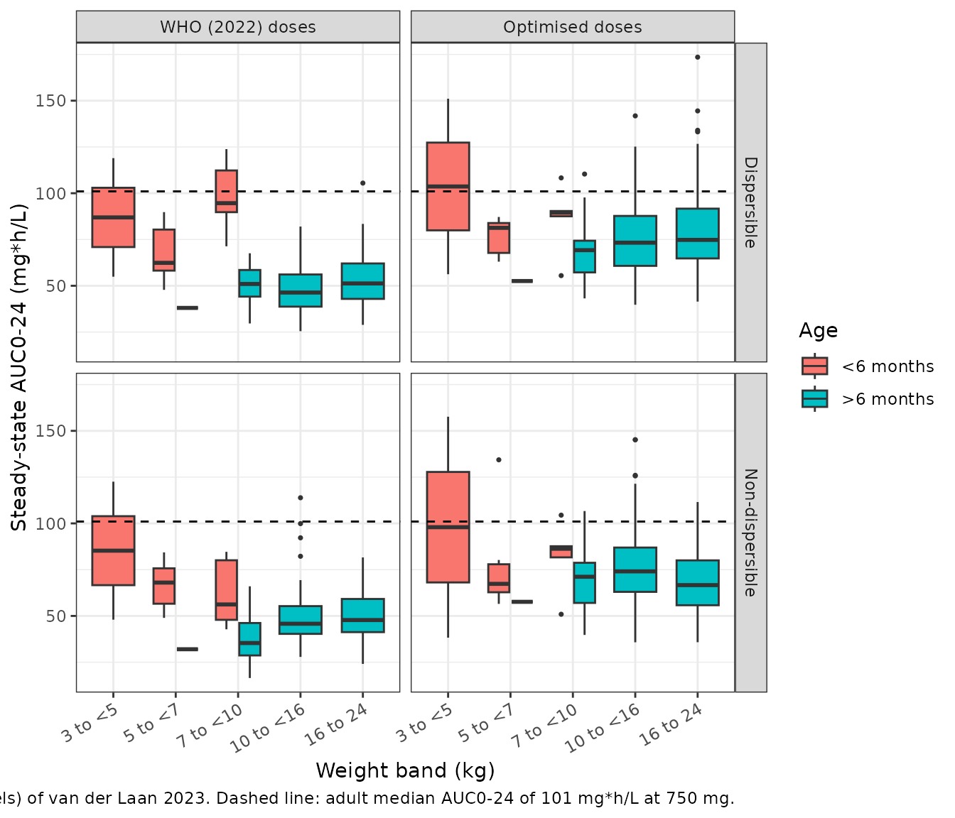
fig_exp |>
  dplyr::filter(regimen == "Optimised doses") |>
  ggplot(aes(band, cmax, fill = age_group)) +
  geom_boxplot(outlier.size = 0.6) +
  geom_hline(yintercept = 14.35, colour = "red") +
  facet_wrap(~formulation) +
  labs(
    x = "Weight band (kg)", y = "Steady-state Cmax (mg/L)", fill = "Age",
    caption = "Replicates Figure 2 (right panels) of van der Laan 2023. Red line: adult median Cmax of 14.35 mg/L at 1000 mg."
  ) +
  theme_bw() +
  theme(axis.text.x = element_text(angle = 30, hjust = 1))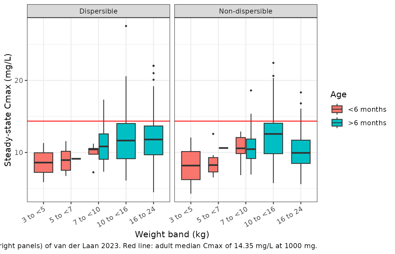
fig_med <- fig_exp |>
  dplyr::filter(!young) |>
  dplyr::group_by(formulation, regimen) |>
  dplyr::summarise(
    n = dplyr::n(),
    median_auc = stats::median(auc),
    pct_auc_ge_101 = 100 * mean(auc >= 101),
    median_cmax = stats::median(cmax),
    .groups = "drop"
  )
fig_med |>
  dplyr::mutate(dplyr::across(c(median_auc, pct_auc_ge_101, median_cmax), \(x) round(x, 1))) |>
  dplyr::rename(
    "Formulation" = formulation, "Regimen" = regimen, "N (>6 months)" = n,
    "Median AUC0-24 (mg*h/L)" = median_auc, "% with AUC >= 101" = pct_auc_ge_101,
    "Median Cmax (mg/L)" = median_cmax
  ) |>
knitr::kable(caption = "Simulated exposure in children over 6 months, pooled across weight bands.")| Formulation | Regimen | N (>6 months) | Median AUC0-24 (mg*h/L) | % with AUC >= 101 | Median Cmax (mg/L) |
|---|---|---|---|---|---|
| Dispersible | WHO (2022) doses | 187 | 49.3 | 0.5 | 7.7 |
| Dispersible | Optimised doses | 187 | 72.9 | 10.7 | 11.4 |
| Non-dispersible | WHO (2022) doses | 187 | 46.2 | 0.5 | 7.3 |
| Non-dispersible | Optimised doses | 187 | 69.3 | 8.0 | 10.8 |
# Cohort-level checks on the centre of the distribution only. The WHO medians
# sit near 50 mg*h/L in Figure 2, and the optimised ones near 75; a dose,
# formulation or clearance error moves these by tens of percent.
who_med <- fig_med$median_auc[fig_med$regimen == "WHO (2022) doses"]
opt_med <- fig_med$median_auc[fig_med$regimen == "Optimised doses"]
stopifnot(all(who_med > 35 & who_med < 75), all(opt_med > 55 & opt_med < 100))
The simulated medians reproduce the pattern of Figure 2. In children over 6 months the pooled median AUC0-24 at WHO doses is about half the adult reference. The optimised doses lift it to roughly 70% of the reference, with median Cmax below the red line. Infants under 6 months, whose clearance is still maturing, reach higher exposures from the same weight-band dose. The paper reports the same picture: “median exposures below adult-equivalent exposures … mainly in children >6 months”, with optimised medians still below 101 mg*h/L (Figure 2, middle panels).
Trial replication and PKNCA
The crossover is simulated in a cohort shaped like Table 1: 150 children, age log-normal around the 2.56-year median (IQR 1.58-4.03), truncated to 0.16-6.01 years, and weight around the WHO median for age, truncated to 4.02-20.3 kg. Each child gets 17.5 mg/kg rounded to 25 mg (the middle of the 15-20 mg/kg target) of each formulation on consecutive days, in randomised order. Day 1 is occasion 2 and day 2 is occasion 3.
set.seed(37596982)
n_trial <- 150
trial_kids <- tibble::tibble(
  AGE = exp(stats::rnorm(4 * n_trial, log(2.56), 0.694))
) |>
  dplyr::filter(AGE >= 0.16, AGE <= 6.01) |>
  dplyr::mutate(WT = who_median_wt(AGE) * exp(stats::rnorm(dplyr::n(), 0, 0.13))) |>
  dplyr::filter(WT >= 4.02, WT <= 20.3) |>
  dplyr::slice_head(n = n_trial) |>
  dplyr::mutate(
    id = dplyr::row_number(),
    dose = pmax(25, round(17.5 * WT / 25) * 25),
    seq_disp_first = stats::rbinom(dplyr::n(), 1, 0.5)
  )
stopifnot(nrow(trial_kids) == n_trial)
summary(trial_kids[, c("AGE", "WT", "dose")])
#>       AGE               WT              dose
#>  Min.   :0.5224   Min.   : 6.078   Min.   :100.0
#>  1st Qu.:1.4751   1st Qu.:10.331   1st Qu.:175.0
#>  Median :2.2845   Median :12.461   Median :225.0
#>  Mean   :2.5070   Mean   :12.697   Mean   :221.3
#>  3rd Qu.:3.3233   3rd Qu.:14.567   3rd Qu.:250.0
#>  Max.   :5.8422   Max.   :19.923   Max.   :350.0

trial_grid <- sort(unique(c(seq(0, 24, by = 0.25), 1, 2, 4, 6, 8)))
ev_trial <- dplyr::bind_rows(
  trial_kids |> tidyr::crossing(period = 1:2) |>
    dplyr::transmute(id, time = 24 * (period - 1), amt = dose, evid = 1, cmt = "depot", period,
      WT, AGE, seq_disp_first),
  # The 24-h sample belongs to period 2 so that the occasion and formulation
  # covariates switch exactly at the day-2 dose; it still closes period 1 in
  # the NCA below (a dose into the depot does not move Cc instantaneously).
  trial_kids |> tidyr::crossing(period = 1:2, tpd = trial_grid) |>
    dplyr::filter(!(period == 1 & tpd == 24)) |>
    dplyr::transmute(id, time = 24 * (period - 1) + tpd, amt = 0, evid = 0, cmt = "central",
      period, WT, AGE, seq_disp_first)
) |>
  dplyr::mutate(
    OCC = period + 1,
    FORM_LEVOFLOXACIN_NONDISPERSIBLE = ifelse((period == 1) == (seq_disp_first == 1), 0, 1)
  ) |>
  dplyr::arrange(id, time, dplyr::desc(evid))

sim_trial <- as.data.frame(rxode2::rxSolve(mod, ev_trial, returnType = "data.frame"))
sim_trial |>
  dplyr::filter(time <= 8 | (time >= 24 & time <= 32)) |>
  dplyr::mutate(
    tpd = ifelse(time >= 24, time - 24, time),
    formulation = ifelse(FORM_LEVOFLOXACIN_NONDISPERSIBLE == 1, "Non-dispersible (crushed)", "Dispersible")
  ) |>
  dplyr::filter(tpd <= 8) |>
  dplyr::group_by(formulation, tpd) |>
  dplyr::summarise(
    p05 = stats::quantile(Cc, 0.05), p50 = stats::median(Cc), p95 = stats::quantile(Cc, 0.95),
    .groups = "drop"
  ) |>
  ggplot(aes(tpd, p50)) +
  geom_ribbon(aes(ymin = p05, ymax = p95), alpha = 0.25) +
  geom_line() +
  facet_wrap(~formulation) +
  labs(
    x = "Time after dose (h)", y = "Levofloxacin (mg/L)",
    caption = "Simulated 5th, 50th and 95th percentiles; compare with Figure 1 of van der Laan 2023."
  ) +
  theme_bw()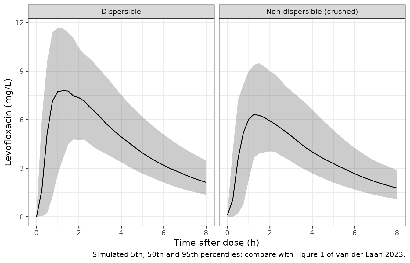
# The 24-h sample closes period 1 and opens period 2; give each period its own
# copy on its own time-after-dose axis.
conc_p1 <- sim_trial |>
  dplyr::filter(time <= 24) |>
  dplyr::mutate(tpd = time)
conc_p2 <- sim_trial |>
  dplyr::filter(time >= 24) |>
  dplyr::mutate(tpd = time - 24)
trt_lookup <- trial_kids |>
  tidyr::crossing(period = 1:2) |>
  dplyr::mutate(treatment = ifelse((period == 1) == (seq_disp_first == 1), "Dispersible", "Non-dispersible")) |>
  dplyr::select(id, period, treatment, dose)
conc_nca <- dplyr::bind_rows(
  dplyr::mutate(conc_p1, period = 1L),
  dplyr::mutate(conc_p2, period = 2L)
) |>
  dplyr::filter(!is.na(Cc)) |>
  dplyr::distinct(id, period, tpd, .keep_all = TRUE) |>
  dplyr::left_join(trt_lookup, by = c("id", "period")) |>
  dplyr::select(id, period, treatment, tpd, Cc)
dose_nca <- trt_lookup |>
  dplyr::mutate(tpd = 0, amt = dose) |>
  dplyr::select(id, period, treatment, tpd, amt)
stopifnot(all(dplyr::count(conc_nca, id, period, tpd)$n == 1))

conc_obj <- PKNCA::PKNCAconc(conc_nca, Cc ~ tpd | treatment + id, concu = "mg/L", timeu = "h")
dose_obj <- PKNCA::PKNCAdose(dose_nca, amt ~ tpd | treatment + id, doseu = "mg")
intervals <- data.frame(start = 0, end = 24, cmax = TRUE, tmax = TRUE, auclast = TRUE)
nca_res <- PKNCA::pk.nca(PKNCA::PKNCAdata(conc_obj, dose_obj, intervals = intervals))
nca_tab <- as.data.frame(nca_res$result)
summary(nca_res)
#>  Interval Start Interval End       treatment   N AUClast (h*mg/L) Cmax (mg/L)
#>               0           24     Dispersible 150      50.0 [24.9] 8.17 [25.7]
#>               0           24 Non-dispersible 150      40.8 [27.0] 6.58 [25.0]
#>            Tmax (h)
#>  1.25 [0.500, 3.00]
#>  1.50 [0.500, 3.25]
#>
#> Caption: AUClast, Cmax: geometric mean and geometric coefficient of variation; Tmax: median and range; N: number of subjects
Comparison against the published exposure
The paper reports one exposure figure from this study: a dispersible-tablet AUC0-24 of 60.0 mgh/L (Discussion, compared against 89.3 mgh/L in an earlier study). The non-dispersible value is not printed; the Table 2 effect implies 78.5% of the dispersible value at equal dose.
reference <- data.frame(treatment = "Dispersible", auclast = 60.0)
cmp <- nlmixr2lib::ncaComparisonTable(
  simulated = nca_tab |>
    dplyr::filter(PPTESTCD %in% c("auclast"), treatment == "Dispersible") |>
    dplyr::select(treatment, PPTESTCD, PPORRES),
  reference = reference,
  by = "treatment",
  units = c(auclast = "mg*h/L")
)
knitr::kable(cmp, caption = "Simulated median versus published dispersible-tablet AUC0-24.")| NCA parameter | treatment | Reference | Simulated | % diff |
|---|---|---|---|---|
| AUClast (mg*h/L) | Dispersible | 60 | 50.3 | -16.2% |
attr(cmp, "footnote")
#> NULL
auc_wide <- nca_tab |>
  dplyr::filter(PPTESTCD == "auclast") |>
  dplyr::select(id, treatment, PPORRES) |>
  tidyr::pivot_wider(names_from = treatment, values_from = PPORRES)
ratio <- auc_wide$`Non-dispersible` / auc_wide$Dispersible
gm_ratio <- exp(mean(log(ratio)))
c(geometric_mean_ratio = gm_ratio, median_disp_auc = stats::median(auc_wide$Dispersible))
#> geometric_mean_ratio      median_disp_auc
#>            0.8151799           50.2916888
# Within-child ratio of two occasions: its log SD is about 0.32 from the F
# BOV, so the geometric mean of 150 ratios has a standard error near 2.6%.
# A wrong sign or a dropped formulation effect moves it by >= 20%.
stopifnot(abs(log(gm_ratio / 0.785)) < 0.10)
# Centre only: the dispersible median sits near 50 mg*h/L in this cohort.
stopifnot(stats::median(auc_wide$Dispersible) > 35, stats::median(auc_wide$Dispersible) < 75)
The simulated dispersible-tablet median AUC0-24 is somewhat below the 60.0 mg*h/L the paper reports. The doses here are a fixed 17.5 mg/kg; the trial doses are only described as “as close to 15-20 mg/kg”, and the virtual weight-for-age relation is approximate. The comparison is shown for information and is not asserted on.
Assumptions and deviations
- Allometric exponents. The Methods state that allometric scaling was applied to all clearance and volume parameters (citing Anderson and Holford) but do not print the exponents. The standard 0.75 for clearances and 1 for volumes are used, as in the parent model (Denti 2018 levofloxacin) from which this analysis started. The reference weight is the cohort median, 12.2 kg (Table 2 footnote).
- Postmenstrual age. Gestational age is not reported. Postmenstrual age is taken as postnatal age plus 9 months, the assumption the parent model states. This agrees with the Discussion’s “half its mature value at ~4 months (~13 months post-menstrual age)” for TM50 = 12.7 months.
-
Maturation is not renormalised. The Table 2
footnote qualifies the typical values by weight only, so
lclis the fully mature clearance at 12.2 kg and the maturation factor tends to 1. At the cohort median age of 2.56 years the factor is 0.989, so the alternative reading (CL normalised to the median age) differs by 1.1%. -
Variability scale. Table 2 prints each variability
as a percentage. It is taken here as
sqrt(omega^2) * 100, the convention of this research group’s levofloxacin and antiretroviral analyses whose control streams are public (Sawe 2025 levofloxacin, Tsirizani 2025 ritonavir). The log-normal CV reading would give a materially smaller variance only for the 98.2% BOV on MTT. -
Occasions. Occasion 1 is the routine dose taken
before the first pharmacokinetic day, seen only through the pre-dose
sample. Its BOV standard deviation on F is 3.24 times the study-dose
value (Table 2). Occasions 2 and 3 are the two study doses. Set
OCC = 0to simulate without between-occasion variability. - Routine formulation. The routine (Austell) tablets given outside the pharmacokinetic days were first modelled separately with parameters fixed to earlier values (Results). The paper does not report a separate bioavailability for them in the final model, so routine doses here take the dispersible reference with the inflated occasion-1 variability.
-
Transit chain written as ODEs. The Savic transit
input, with N fixed to 10, is encoded as an explicit chain: the dose
compartment
depotandtransit1totransit10empty at ktr = 11 / MTT into the absorption compartmenttransit11, which empties intocentralat ka. This is mathematically identical to the analytical Savic input. It is used instead of rxode2’stransit()because the 98% between-occasion variability on MTT produces some very short MTTs, for which the analytical input is a spike the ODE solver can step over and lose the dose. Doses go todepot. - Residual error. The combined additive and proportional error uses the Table 2 values. The paper does not state whether an LLOQ-based floor was added to the additive term, so none is added. Below-LLOQ handling (Beal M3) is a fitting device and is not part of the simulation model.
- Virtual cohorts. Weights come from an approximate WHO median weight-for-age curve with a 13% spread, not from the tuberculosis-specific in silico population used for the paper’s dosing simulations. Assertions on the stochastic cohorts are on medians and geometric means only.