Carbamazepine (Yip 2021)
Source:vignettes/articles/Yip_2021_carbamazepine.Rmd
Yip_2021_carbamazepine.RmdModel and source
#> ℹ parameter labels from comments will be replaced by 'label()'- Citation: Yip VLM, Pertinez H, Meng X, Maggs JL, Carr DF, Park BK, Marson AG, Pirmohamed M. Evaluation of clinical and genetic factors in the population pharmacokinetics of carbamazepine. Br J Clin Pharmacol. 2021;87(6):2572-2588. doi:10.1111/bcp.14667
- Description: Simultaneous parent + three-metabolite population PK model for carbamazepine (CBZ) and its metabolites carbamazepine-10,11-epoxide (CBZE), 2-hydroxycarbamazepine (2OH-CBZ) and 3-hydroxycarbamazepine (3OH-CBZ) in healthy adult volunteers and adults with epilepsy (Yip 2021). One-compartment parent with first-order absorption and elimination feeding three metabolite compartments that share one apparent volume of distribution (an identifiability assumption); total apparent parent clearance partitioned via a fixed metabolite fraction into CBZE, 2OH-CBZ and 3OH-CBZ formation. Covariates: binary enzyme-autoinduction status (>= 14 days of dosing) on total clearance and on 2OH-CBZ elimination, phenytoin coadministration and total daily carbamazepine dose on total clearance, and the EPHX1 rs2234922 homozygous-variant (416G/G) genotype on CBZE elimination. Concentrations are molar (mmol/L); all clearances and volumes are apparent (CL/F, V/F) because no intravenous data were available.
- Article: https://doi.org/10.1111/bcp.14667
Population
Yip 2021 fit a simultaneous parent-plus-three-metabolite population PK model to 80 adults studied in two UK trials: PICME I (8 healthy male volunteers given a single 400 mg oral immediate-release carbamazepine dose with rich sampling to 72 h) and PICME II (epilepsy patients – an autoinduction group of 3 patients titrated from 200 mg once daily to 200 mg AM / 400 mg PM over 42 days, and a maintenance group of 69 patients on stable therapy, 819 +/- 367 mg/day, with sparse sampling). In total 248 sets of carbamazepine (CBZ) + metabolite assays were used. The three metabolites modelled are the active, chemically reactive carbamazepine-10,11-epoxide (CBZE), 2-hydroxycarbamazepine (2OH-CBZ) and 3-hydroxycarbamazepine (3OH-CBZ). Age ranged 21.7-75.8 years (mean 45.8) and weight 39.0-140.5 kg (mean 80.8); see Yip 2021 Table 3 for the full demographics and Table 4 for the genotype distribution.
The same metadata is available programmatically via
readModelDb("Yip_2021_carbamazepine")()$population.
Model structure
A one-compartment parent (first-order absorption and elimination)
feeds three metabolite compartments that share a single apparent volume
of distribution V2 (an identifiability assumption; Yip 2021 Methods
2.8). The total apparent parent clearance CLTOT is partitioned (Eqs 6-8)
into formation of the three metabolites: a fraction
1 - FM1 = 0.36 forms CBZE and FM1/2 = 0.32
each forms 2OH-CBZ and 3OH-CBZ, with FM1 fixed at 0.64 for
identifiability. Each metabolite is eliminated first-order (CL2E, CL3E,
CL4E). The absorption rate is constrained above the parent elimination
rate via KA = CLTOT/V1 + KAstar (Eq 9) to avoid flip-flop.
Concentrations are molar (mmol/L); a carbamazepine dose in mg is
converted with the molecular weight 236.27 g/mol.
Covariates in the final model: a binary enzyme-autoinduction status on CLTOT (x1.73) and on 2OH-CBZ elimination clearance (x1.63); phenytoin coadministration (x1.93) and total daily dose (an additive log term) on CLTOT; and the EPHX1 rs2234922 homozygous-variant (416G/G) genotype on CBZE elimination clearance (x0.502).
Source trace
The per-parameter origin is recorded as an in-file comment next to
each ini() entry in
inst/modeldb/specificDrugs/Yip_2021_carbamazepine.R. The
table below collects them in one place for review. All point estimates
are from Yip 2021 Table 5.
| Equation / parameter | Value | Source location |
|---|---|---|
lcl (CLTOT, total apparent clearance) |
1.96 L/h | Table 5 |
lvc (V1, parent central volume) |
161 L | Table 5 |
lkastar (KAstar absorption offset) |
0.409 /h | Table 5; Eq 9 |
lfm1 (FM1, fraction to hydroxy metabolites) |
0.64 (FIXED) | Table 5 + Methods 2.8 |
lcl_cbze (CL2E, CBZE elimination) |
9.71 L/h | Table 5 |
lcl_2oh (CL3E, 2OH-CBZ elimination) |
726 L/h | Table 5 |
lcl_3oh (CL4E, 3OH-CBZ elimination) |
543 L/h | Table 5 |
lvc_met (V2, shared metabolite volume) |
39.2 L | Table 5 |
e_autoind_cl (autoinduction on CLTOT) |
1.73 | Table 5; Eq 17 |
e_autoind_cl_2oh (autoinduction on CL3E) |
1.63 | Table 5; Eq 18 |
e_pht_cl (phenytoin on CLTOT) |
1.93 | Table 5; Eq 17 |
e_dose_cl (daily dose on CLTOT, additive ln term) |
1.36 | Table 5; Eqs 13, 17 |
e_ephx1_hom_cl_cbze (EPHX1 416G/G on CBZE elim) |
0.502 | Table 5; see Errata re Eq 18 |
| IIV CV% (Table 5) | CLTOT 25.3, FM1 6.3, CL2E 27.9, CL3E 42.3, CL4E 34.5, KASTAR 75.3, V1 13.6, V2 149.7 | Table 5; converted via omega^2 = log(1 + CV^2) |
| Exponential residual SD | CBZ 0.221, CBZE 0.310, 2OH-CBZ 0.297, 3OH-CBZ 0.362 | Table 5 |
d/dt(central) + 3 metabolite ODEs |
n/a | Eqs 1-9, Figure 2 |
Virtual cohort
Original observed data are not publicly available. The cohort simulated here reproduces the PICME I design – a single 400 mg oral immediate-release dose in non-induced, phenytoin-free, EPHX1 wild-type subjects – with between-subject variability on all structural parameters. Carbamazepine molecular weight 236.27 g/mol is used to convert the 400 mg dose to 1.693 mmol.
set.seed(20260829L)

mw_cbz <- 236.27
dose_mg <- 400
dose_mmol <- dose_mg / mw_cbz

# Observation grid: dense through absorption / distribution, then out to
# 336 h (about 6 parent half-lives) so AUCinf extrapolation is small.
obs_times <- sort(unique(c(
  seq(0, 24, by = 0.5),
  seq(26, 72, by = 2),
  seq(80, 336, by = 8)
)))

# Build one arm as a self-contained event table. This is a four-endpoint model
# (Cc, Cc_cbze, Cc_2oh, Cc_3oh), so observation rows carry the ODE state name
# `central` plus `dvid = 1L` (NOT `cmt = "Cc"`, which would target an auto-
# injected endpoint slot); rxode2 still returns every observable as a column at
# those rows. Dose rows carry `dvid = NA_integer_`.
make_arm <- function(n, autoind, pht, ephx_hom, dose_mgd,
                     dose_amt = dose_mmol, id_offset = 0L) {
  ids <- id_offset + seq_len(n)
  covs <- function(k) {
    tibble(
      AUTOIND_STATUS = autoind,
      CONMED_PHT = pht,
      SNP_EPHX1_RS2234922_HOM = ephx_hom,
      DOSE_CBZ_MGD = dose_mgd
    )[rep(1, k), ]
  }
  dose_rows <- bind_cols(
    tibble(
      id = ids, time = 0, evid = 1L, amt = dose_amt,
      cmt = "depot", dvid = NA_integer_
    ),
    covs(n)
  )
  obs_rows <- bind_cols(
    tibble(
      id = rep(ids, each = length(obs_times)),
      time = rep(obs_times, times = n),
      evid = 0L, amt = NA_real_, cmt = "central", dvid = 1L
    ),
    covs(n * length(obs_times))
  )
  bind_rows(dose_rows, obs_rows) |>
    arrange(id, time, desc(evid))
}

n_sub <- 200L
events <- make_arm(
  n = n_sub, autoind = 0, pht = 0, ephx_hom = 0, dose_mgd = 400
)
stopifnot(!anyDuplicated(unique(events[, c("id", "time", "evid")])))
Simulation
mod <- readModelDb("Yip_2021_carbamazepine")

# useLinCmt = FALSE: this is a multi-output, multi-state model; the explicit
# ODE path is the validation (default since the 2026-09-24 rxode2 build).
sim <- rxode2::rxSolve(mod, events = events, useLinCmt = FALSE) |>
  as.data.frame() |>
  as_tibble()
#> ℹ parameter labels from comments will be replaced by 'label()'
Replicate the four-analyte concentration-time profiles (Figures 3-4)
Yip 2021 Figures 3 (goodness-of-fit) and 4 (prediction-corrected VPC) show the CBZ, CBZE, 2OH-CBZ and 3OH-CBZ concentration-time behaviour in mmol/L. The prediction interval below is the simulated 5th-50th-95th percentile envelope for each analyte after a single 400 mg dose.
sim_long <- sim |>
  filter(time > 0) |>
  select(id, time, Cc, Cc_cbze, Cc_2oh, Cc_3oh) |>
  pivot_longer(
    c(Cc, Cc_cbze, Cc_2oh, Cc_3oh),
    names_to = "analyte", values_to = "conc"
  ) |>
  mutate(analyte = recode(analyte,
    Cc = "CBZ", Cc_cbze = "CBZE",
    Cc_2oh = "2OH-CBZ", Cc_3oh = "3OH-CBZ"
  ))

vpc <- sim_long |>
  filter(conc > 0) |>
  group_by(analyte, time) |>
  summarise(
    Q05 = quantile(conc, 0.05, na.rm = TRUE),
    Q50 = quantile(conc, 0.50, na.rm = TRUE),
    Q95 = quantile(conc, 0.95, na.rm = TRUE),
    .groups = "drop"
  )

ggplot(vpc, aes(time, Q50)) +
  geom_ribbon(aes(ymin = Q05, ymax = Q95), alpha = 0.25) +
  geom_line() +
  facet_wrap(~analyte, scales = "free_y") +
  scale_x_continuous(limits = c(0, 168)) +
  labs(
    x = "Time after a single 400 mg oral dose (h)",
    y = "Concentration (mmol/L)",
    title = "Simulated 5-50-95% envelope for CBZ and its three metabolites",
    caption = "Reproduces the analyte structure of Yip 2021 Figures 3-4 (single 400 mg dose, non-induced)."
  ) +
  theme_bw()
#> Warning: Removed 84 rows containing missing values or values outside the scale range
#> (`geom_ribbon()`).
#> Warning: Removed 84 rows containing missing values or values outside the scale range
#> (`geom_line()`).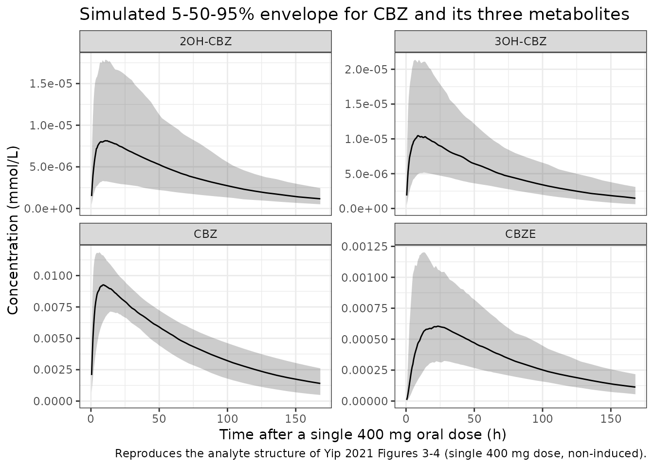
Closed-form validation of the clearance partition and covariate effects
For a single oral dose with complete (apparent) bioavailability, the
parent AUC to infinity equals Dose / CLTOT independent of
absorption rate, and by mass balance each metabolite’s AUC to infinity
equals
(formation fraction x Dose) / (metabolite elimination clearance).
These identities let the simulated NCA pin every structural and
covariate value exactly, with no tuning. The checks below use
typical-value simulations (zeroRe()), so any discrepancy is
pure numerical-integration error.
mod_typ <- mod |> rxode2::zeroRe()
#> ℹ parameter labels from comments will be replaced by 'label()'

solve_typ <- function(autoind, pht, ephx_hom, dose_mgd) {
  ev <- make_arm(
    n = 1, autoind = autoind, pht = pht, ephx_hom = ephx_hom,
    dose_mgd = dose_mgd
  )
  rxode2::rxSolve(mod_typ, events = ev, useLinCmt = FALSE) |>
    as.data.frame() |>
    as_tibble()
}

# AUCinf of a single analyte from a typical-value profile, via PKNCA.
aucinf_of <- function(df, conc_col) {
  d <- df |>
    transmute(id = 1L, time = time, conc = .data[[conc_col]]) |>
    filter(!is.na(conc))
  d <- bind_rows(tibble(id = 1L, time = 0, conc = 0), d) |>
    distinct(id, time, .keep_all = TRUE) |>
    arrange(time)
  co <- PKNCA::PKNCAconc(d, conc ~ time | id)
  do <- PKNCA::PKNCAdose(
    data.frame(id = 1L, time = 0, amt = dose_mmol), amt ~ time | id
  )
  iv <- data.frame(start = 0, end = Inf, aucinf.obs = TRUE)
  res <- PKNCA::pk.nca(PKNCA::PKNCAdata(co, do, intervals = iv))
  r <- as.data.frame(res$result)
  r$PPORRES[r$PPTESTCD == "aucinf.obs"]
}

# Reference (non-induced, no PHT, wild-type, 400 mg/day) --------------------
ref <- solve_typ(autoind = 0, pht = 0, ephx_hom = 0, dose_mgd = 400)
#> ℹ omega/sigma items treated as zero: 'etalcl', 'etalfm1', 'etalcl_cbze', 'etalcl_2oh', 'etalcl_3oh', 'etalkastar', 'etalvc', 'etalvc_met'

fm1 <- 0.64
auc_parent_obs <- aucinf_of(ref, "Cc")
auc_cbze_obs <- aucinf_of(ref, "Cc_cbze")
auc_2oh_obs <- aucinf_of(ref, "Cc_2oh")
auc_3oh_obs <- aucinf_of(ref, "Cc_3oh")

auc_parent_cf <- dose_mmol / 1.96
auc_cbze_cf <- (1 - fm1) * dose_mmol / 9.71
auc_2oh_cf <- (fm1 / 2) * dose_mmol / 726
auc_3oh_cf <- (fm1 / 2) * dose_mmol / 543

closed_form <- tibble(
  Analyte = c("CBZ (parent)", "CBZE", "2OH-CBZ", "3OH-CBZ"),
  `Closed form` = c(auc_parent_cf, auc_cbze_cf, auc_2oh_cf, auc_3oh_cf),
  `Simulated NCA` = c(auc_parent_obs, auc_cbze_obs, auc_2oh_obs, auc_3oh_obs)
) |>
  mutate(`% diff` = 100 * (`Simulated NCA` - `Closed form`) / `Closed form`)

knitr::kable(
  closed_form,
  caption = "AUCinf (mmol*h/L) after a single 400 mg dose: closed-form mass balance vs simulated NCA.",
  digits = 6
)| Analyte | Closed form | Simulated NCA | % diff |
|---|---|---|---|
| CBZ (parent) | 0.863764 | 0.863687 | -0.008927 |
| CBZE | 0.062767 | 0.062772 | 0.006662 |
| 2OH-CBZ | 0.000746 | 0.000746 | -0.003593 |
| 3OH-CBZ | 0.000998 | 0.000998 | -0.002397 |
# Numerical-integration / tail-extrapolation error only (measured <= 0.01%);
# a mis-transcribed clearance, fraction or dose would move these by tens of
# percent.
stopifnot(all(abs(closed_form$`% diff`) < 0.5))
# Each covariate is a power-of-binary (or additive-ln) multiplier whose effect
# on an AUC is an exact ratio under the mass-balance identities above.
auc_parent <- function(df) aucinf_of(df, "Cc")
auc_cbze <- function(df) aucinf_of(df, "Cc_cbze")

# Autoinduction raises CLTOT 1.73x, so parent AUC falls to 1/1.73 (ratio 1.73).
induced <- solve_typ(autoind = 1, pht = 0, ephx_hom = 0, dose_mgd = 400)
#> ℹ omega/sigma items treated as zero: 'etalcl', 'etalfm1', 'etalcl_cbze', 'etalcl_2oh', 'etalcl_3oh', 'etalkastar', 'etalvc', 'etalvc_met'
ratio_autoind <- auc_parent(ref) / auc_parent(induced)

# Phenytoin raises CLTOT 1.93x.
pht <- solve_typ(autoind = 0, pht = 1, ephx_hom = 0, dose_mgd = 400)
#> ℹ omega/sigma items treated as zero: 'etalcl', 'etalfm1', 'etalcl_cbze', 'etalcl_2oh', 'etalcl_3oh', 'etalkastar', 'etalvc', 'etalvc_met'
ratio_pht <- auc_parent(ref) / auc_parent(pht)

# Total daily dose enters CLTOT additively as ln((DOSE/400)^1.36). At
# DOSE = 800, CLTOT = 1.96 + ln((800/400)^1.36) = 1.96 + 1.36*ln(2).
dose800 <- solve_typ(autoind = 0, pht = 0, ephx_hom = 0, dose_mgd = 800)
#> ℹ omega/sigma items treated as zero: 'etalcl', 'etalfm1', 'etalcl_cbze', 'etalcl_2oh', 'etalcl_3oh', 'etalkastar', 'etalvc', 'etalvc_met'
cltot_800 <- 1.96 + 1.36 * log(2)
ratio_dose_cf <- cltot_800 / 1.96
ratio_dose_obs <- auc_parent(ref) / auc_parent(dose800)

# EPHX1 416G/G lowers CBZE elimination clearance to 0.502x, so CBZE AUC rises
# to 1/0.502 = 1.992.
ephx <- solve_typ(autoind = 0, pht = 0, ephx_hom = 1, dose_mgd = 400)
#> ℹ omega/sigma items treated as zero: 'etalcl', 'etalfm1', 'etalcl_cbze', 'etalcl_2oh', 'etalcl_3oh', 'etalkastar', 'etalvc', 'etalvc_met'
ratio_ephx_cbze <- auc_cbze(ephx) / auc_cbze(ref)

ratios <- tibble(
  Effect = c(
    "Autoinduction on CLTOT (parent AUC ratio)",
    "Phenytoin on CLTOT (parent AUC ratio)",
    "Daily dose 800 vs 400 mg on CLTOT (parent AUC ratio)",
    "EPHX1 416G/G on CBZE elimination (CBZE AUC ratio)"
  ),
  Expected = c(1.73, 1.93, ratio_dose_cf, 1 / 0.502),
  Simulated = c(ratio_autoind, ratio_pht, ratio_dose_obs, ratio_ephx_cbze)
) |>
  mutate(`% diff` = 100 * (Simulated - Expected) / Expected)

knitr::kable(
  ratios,
  caption = "Covariate multipliers recovered as exact AUC ratios (typical-value simulation).",
  digits = 4
)| Effect | Expected | Simulated | % diff |
|---|---|---|---|
| Autoinduction on CLTOT (parent AUC ratio) | 1.730 | 1.7302 | 0.0107 |
| Phenytoin on CLTOT (parent AUC ratio) | 1.930 | 1.9303 | 0.0132 |
| Daily dose 800 vs 400 mg on CLTOT (parent AUC ratio) | 1.481 | 1.4811 | 0.0074 |
| EPHX1 416G/G on CBZE elimination (CBZE AUC ratio) | 1.992 | 1.9920 | -0.0009 |
PKNCA on the stochastic cohort
Yip 2021 does not report a non-compartmental analysis, so the NCA
below characterises the simulated 400 mg single-dose cohort for all four
analytes. The parent terminal half-life recovers
log(2) * V1 / CLTOT.
sim_nca <- sim |>
  filter(!is.na(Cc)) |>
  select(id, time, Cc, Cc_cbze, Cc_2oh, Cc_3oh)

# Guarantee a time = 0 row per subject (pre-dose extravascular conc = 0).
zero_rows <- sim_nca |>
  distinct(id) |>
  mutate(time = 0, Cc = 0, Cc_cbze = 0, Cc_2oh = 0, Cc_3oh = 0)

sim_nca <- bind_rows(sim_nca, zero_rows) |>
  distinct(id, time, .keep_all = TRUE) |>
  arrange(id, time)

dose_df <- events |>
  filter(evid == 1L) |>
  select(id, time, amt)
dose_obj <- PKNCA::PKNCAdose(dose_df, amt ~ time | id)

intervals <- data.frame(
  start = 0, end = Inf,
  cmax = TRUE, tmax = TRUE, aucinf.obs = TRUE, half.life = TRUE
)

nca_one <- function(conc_col) {
  co <- PKNCA::PKNCAconc(sim_nca, stats::as.formula(paste(conc_col, "~ time | id")))
  res <- PKNCA::pk.nca(PKNCA::PKNCAdata(co, dose_obj, intervals = intervals))
  as.data.frame(res$result) |>
    group_by(PPTESTCD) |>
    summarise(median = median(PPORRES, na.rm = TRUE), .groups = "drop") |>
    pivot_wider(names_from = PPTESTCD, values_from = median) |>
    mutate(Analyte = conc_col)
}

nca_tab <- bind_rows(lapply(
  c("Cc", "Cc_cbze", "Cc_2oh", "Cc_3oh"), nca_one
)) |>
  mutate(Analyte = recode(Analyte,
    Cc = "CBZ", Cc_cbze = "CBZE", Cc_2oh = "2OH-CBZ", Cc_3oh = "3OH-CBZ"
  )) |>
  select(Analyte, cmax, tmax, aucinf.obs, half.life)

knitr::kable(
  nca_tab,
  caption = "Simulated NCA (cohort medians) after a single 400 mg oral dose.",
  digits = 5
)| Analyte | cmax | tmax | aucinf.obs | half.life |
|---|---|---|---|---|
| CBZ | 0.00945 | 8.75 | 0.86950 | 55.96536 |
| CBZE | 0.00064 | 19.00 | 0.06493 | 56.97512 |
| 2OH-CBZ | 0.00001 | 9.00 | 0.00076 | 55.96621 |
| 3OH-CBZ | 0.00001 | 9.00 | 0.00094 | 55.96653 |
# Parent terminal half-life should recover log(2) * V1 / CLTOT = 56.9 h. This
# is a cohort median (measured 56.0 h), so the bound allows for which subjects
# are drawn; a wrong V1 or CLTOT shifts it by tens of percent.
hl_parent_cf <- log(2) * 161 / 1.96
hl_parent_sim <- nca_tab$half.life[nca_tab$Analyte == "CBZ"]
stopifnot(abs(hl_parent_sim - hl_parent_cf) / hl_parent_cf < 0.10)
Assumptions and deviations
EPHX1 covariate placed on CBZE elimination (CL2E), not CL3E. The printed Equation 18 of Yip 2021 attaches the EPHX1 416G/G (EPHXAGHOM) effect to CL3E (the 2OH-CBZ elimination clearance). Every other statement of the result places it on CBZE elimination: Table 5 reads
Cov.Eff.(EPHXAGHOM on CL2E) 0.502, Table 6 readsEPHXAGHOM on CL2E, Methods 2.8 states the EPHX genotypes were “investigated for potential effects on CL2E as these genes are specifically associated with the metabolic clearance of CBZE”, and the Discussion states “their clearance of CBZE was reduced by approximately 50%”. The maintainers encode the effect on CBZE elimination (CL2E) and treat the “CL3E” in Equation 18 as a transcription artifact. CL3E carries only the autoinduction effect (Equation 11).Total daily dose enters clearance additively on the log scale. Equations 13 and 17 add
ln((DOSE/400)^1.36)to the typical CLTOT rather than multiplying by a power term. This is reproduced exactly; the term vanishes at the 400 mg/day reference dose.IIV reported as CV%, converted to log-normal variance. Table 5 gives interindividual variability as a percentage for each log-normal random effect; the model stores
omega^2 = log(1 + CV^2). The CV%-vs-apparent-CV convention is not stated in the paper; the mathematically exact log-normal conversion is used. This mainly affects V2, whose 149.7% CV is poorly estimated (ETA-shrinkage 64%); its large nominal IIV is retained for fidelity but contributes little information.FM1 fixed at 0.64 with a small estimated IIV. FM1 is fixed to 0.64 for identifiability (36% of CBZ converts primarily to CBZE, from prior mass balance), but Table 5 still reports a 6.3% IIV on it (ETA-shrinkage 65%). The typical value is wrapped in
fixed()while the small IIV is retained.Mole-for-mole metabolite stoichiometry. All analytes are modelled in molar units, so each formation flux carries parent moles into metabolite moles 1:1 with no molecular-weight correction, matching the paper’s molar parameterisation.
Apparent (CL/F, V/F) parameters. No intravenous data were available, so every clearance and volume is apparent; absolute bioavailability is not identifiable and is treated as 1.
Interoccasion variability omitted. Yip 2021 attempted IOV but it “failed to produce acceptable fittings”, so none is implemented.
No correction notice. No erratum or corrigendum to Yip 2021 was located as of the maintainers’ literature check (2026-10-16); the single internal inconsistency (Equation 18) is resolved above from the paper’s own tables and text.