Aflibercept free and bound MM-TMDD (Thai 2011)
Source:vignettes/articles/Thai_2011_aflibercept.Rmd
Thai_2011_aflibercept.RmdModel and source
- Citation: Thai HT, Veyrat-Follet C, Vivier N, Dubruc C, Sanderink G, Mentre F, Comets E. A mechanism-based model for the population pharmacokinetics of free and bound aflibercept in healthy subjects. Br J Clin Pharmacol. 2011;72(3):402-414. doi:10.1111/j.1365-2125.2011.04015.x
- Description: Mechanism-based population PK model for free and bound aflibercept (anti-VEGF Fc-fusion ‘trap’ protein; VEGF-Trap) in healthy adult male subjects (Thai 2011 BJCP). Two-compartment disposition of free aflibercept with linear elimination from the central compartment plus Michaelis-Menten binding of free aflibercept to VEGF occurring in the peripheral (tissue) compartment, producing a one-compartment bound-aflibercept species that is eliminated by first-order internalisation (kint). This is the second Michaelis-Menten approximation of the TMDD model of Gibiansky et al. (irreversible binding), with the bound complex carried as an explicit state. The bound-aflibercept volume of distribution Vb is fixed equal to the central volume Vc for identifiability. Pooled data from two phase 1 single-dose IV-infusion studies in healthy males (1, 2, 4 mg/kg over 1 h). No covariates were tested or retained in the final model.
- Article: https://doi.org/10.1111/j.1365-2125.2011.04015.x
The model is the second Michaelis-Menten approximation of the TMDD model of Gibiansky et al. (irreversible-binding form) applied to aflibercept binding to vascular endothelial growth factor (VEGF). The bound complex is carried as an explicit state and eliminated by first-order internalisation (kint). Binding of free aflibercept to VEGF occurs in the peripheral (tissue) compartment, consistent with the paper’s Discussion noting that large quantities of VEGF reside in the extravascular space.
Population
The model was fit to pooled data from two phase 1 single-dose IV-infusion studies in 56 healthy male volunteers (36 from study 1 in South Africa; 20 from study 2 in Germany receiving IV in the first period of a crossover design). Doses were 1, 2 or 4 mg/kg aflibercept administered as a 1 h IV infusion. A total of 1476 concentrations were analysed (732 free aflibercept and 744 bound aflibercept), of which 242 (32.5 %) bound concentrations were below the LOQ of 0.0314 ug eq/mL and were treated using the SAEM censored-data extension in MONOLIX 3.1. No covariates were tested because the population is uniform.
Source trace
The per-parameter origin is also recorded as an in-file comment on
each ini() entry of
inst/modeldb/specificDrugs/Thai_2011_aflibercept.R.
| Equation / parameter | Value | Source location |
|---|---|---|
lcl (CL, L/day) |
0.88 | Table 1 row 1 (RSE 4 %) |
lvc (Vc = Vp paper, L) |
4.94 | Table 1 row 2 (RSE 4 %) |
lq (Q, L/day) |
1.39 | Table 1 row 3 (RSE 9 %) |
lvp (Vp = Vt paper, L) |
2.33 | Table 1 row 4 (RSE 7 %) |
vb derived = vc
|
4.94 | Table 1 row 5: 4.94 (= Vp); main text page 405 |
lvmax (Vmax, mg/day) |
0.99 | Table 1 row 6 (RSE 5 %) |
lkm (Km, ug/mL) |
2.91 | Table 1 row 7 (RSE 11 %) |
lkint (kint, 1/day) |
0.028 | Table 1 row 8 (RSE 5 %) |
etalcl (w on CL) |
28.0 % -> omega^2 = 0.0784 | Table 1 col 3 row 1 |
etalvc (w on Vp) |
27.3 % -> omega^2 = 0.07453 | Table 1 col 3 row 2 |
etalq (w on Q) |
49.8 % -> omega^2 = 0.24800 | Table 1 col 3 row 3 |
etalvp (w on Vt) |
39.8 % -> omega^2 = 0.15840 | Table 1 col 3 row 4 |
etalvmax (w on Vmax) |
13.6 % -> omega^2 = 0.01850 | Table 1 col 3 row 6 |
etalkm (w on Km) |
45.6 % -> omega^2 = 0.20794 | Table 1 col 3 row 7 |
| IIV on kint dropped | n/a | Table 1 col 3 row 8 (-); main text page 405 |
propSd (free) |
0.171 | Table 1 free residual block (RSE 3 %) |
addSd (free, ug/mL) |
0.05 | Table 1 free residual block (RSE 9 %) |
propSd_complex (bound) |
0.126 | Table 1 bound residual block (RSE 4 %) |
| ODE system | n/a | Main text equations page 405; Appendix Eq. A14 |
| MM binding in peripheral | n/a | Main text page 405 (nonlinear peripheral binding chosen by BIC) |
Virtual cohort
The original observed data are not publicly available. The cohort below matches the trial design (Methods, “Study design”): three single-dose IV infusion groups at 1, 2 and 4 mg/kg given over 1 hour, with sampling on day 1 (pre, end-of-infusion, 1, 3, 5, 7, 11 and 23 hours post end-of-infusion – approximately the paper’s 0, 1, 2, 4, 6, 8, 12 and 24 h post start of infusion) and on days 8, 15, 22, 29, 36 and 43. Body weight is set to 75 kg, the typical adult-male reference, because the paper does not enumerate per-subject weights in Table 1 or in the results text; this assumption only affects the absolute mg dose, not the shape of the PK profile.
set.seed(20260613)

ref_wt_kg <- 75                       # assumed adult-male reference weight
infusion_dur_day <- 1 / 24            # 1-hour infusion in day units
n_per_dose <- 30L

# Sampling grid in days: matches the paper's blood sampling schedule for study 1.
# Day 1 times after end of infusion: pre (0), end-of-infusion (1/24), 2/24, 4/24,
# 6/24, 8/24, 12/24, 24/24; then days 8, 15, 22, 29, 36, 43.
day1_grid <- c(0, 1/24, 2/24, 4/24, 6/24, 8/24, 12/24, 1)
late_grid <- c(8, 15, 22, 29, 36, 43)
sample_grid <- sort(unique(c(day1_grid, late_grid,
                             # add interior points so the bound peak is captured
                             seq(0, 60, by = 1))))

make_cohort <- function(dose_mg_per_kg, id_offset) {
  ids <- id_offset + seq_len(n_per_dose)
  amt_mg <- dose_mg_per_kg * ref_wt_kg
  rate_mg_per_day <- amt_mg / infusion_dur_day

  dose_rows <- data.frame(
    id   = ids,
    time = 0,
    amt  = amt_mg,
    rate = rate_mg_per_day,
    evid = 1L,
    cmt  = "central"
  )
  obs_cc <- expand.grid(id = ids, time = sample_grid)
  obs_cc$amt  <- 0
  obs_cc$rate <- 0
  obs_cc$evid <- 0L
  obs_cc$cmt  <- "Cc"

  obs_complex <- obs_cc
  obs_complex$cmt <- "Cc_complex"

  out <- dplyr::bind_rows(dose_rows, obs_cc, obs_complex)
  out$treatment <- sprintf("%s mg/kg", format(dose_mg_per_kg, nsmall = 0))
  out$dose_mg_per_kg <- dose_mg_per_kg
  out[order(out$id, out$time, -out$evid), ]
}

events <- dplyr::bind_rows(
  make_cohort(1, id_offset =   0L),
  make_cohort(2, id_offset = 100L),
  make_cohort(4, id_offset = 200L)
)
stopifnot(!anyDuplicated(unique(events[, c("id", "time", "evid", "cmt")])))
Simulation
mod <- readModelDb("Thai_2011_aflibercept")

# Stochastic simulation with the full IIV (used for Figure 5 / VPC-style plots).
sim_iiv <- rxode2::rxSolve(mod, events = events,
                           keep = c("treatment", "dose_mg_per_kg")) |>
  as.data.frame()
#> ℹ parameter labels from comments will be replaced by 'label()'

# Typical-value (no random effects) for Figure 1-style mean trajectories
mod_typ <- rxode2::zeroRe(mod)
#> ℹ parameter labels from comments will be replaced by 'label()'
sim_typ <- rxode2::rxSolve(mod_typ, events = events,
                           keep = c("treatment", "dose_mg_per_kg")) |>
  as.data.frame()
#> ℹ omega/sigma items treated as zero: 'etalcl', 'etalvc', 'etalq', 'etalvp', 'etalvmax', 'etalkm'
#> Warning: multi-subject simulation without without 'omega'
Replicate published figures
Figure 1A – free aflibercept concentration vs time (semi-log)
# Replicates Figure 1A of Thai 2011: free aflibercept (ug/mL) vs time on a
# semi-log scale, showing the bi-exponential decline at three dose levels.
sim_iiv |>
  dplyr::filter(Cc > 0) |>
  dplyr::group_by(treatment, time) |>
  dplyr::summarise(
    Q05 = stats::quantile(Cc, 0.05, na.rm = TRUE),
    Q50 = stats::quantile(Cc, 0.50, na.rm = TRUE),
    Q95 = stats::quantile(Cc, 0.95, na.rm = TRUE),
    .groups = "drop"
  ) |>
  ggplot(aes(time, Q50, colour = treatment, fill = treatment)) +
  geom_ribbon(aes(ymin = Q05, ymax = Q95), alpha = 0.2, colour = NA) +
  geom_line() +
  scale_y_log10() +
  labs(x = "Time (day)", y = "Free aflibercept (ug/mL)",
       title = "Figure 1A -- free aflibercept vs time",
       caption = "Replicates Figure 1A of Thai 2011. Ribbon = 5-95% sim interval; line = median.") +
  theme(legend.position = "bottom")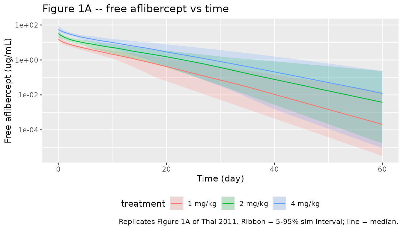
Figure 1B – bound aflibercept concentration vs time (linear)
# Replicates Figure 1B of Thai 2011: bound aflibercept (ug eq/mL) vs time on a
# linear scale. The bound peak occurs around day 21 for the 2 and 4 mg/kg
# doses (Thai 2011, Results, 'The peaks of complex occurred sooner for
# 1 mg/kg and later for doses of 2 and 4 mg/kg (around 21 days for both
# doses).').
sim_iiv |>
  dplyr::filter(Cc_complex > 0) |>
  dplyr::group_by(treatment, time) |>
  dplyr::summarise(
    Q05 = stats::quantile(Cc_complex, 0.05, na.rm = TRUE),
    Q50 = stats::quantile(Cc_complex, 0.50, na.rm = TRUE),
    Q95 = stats::quantile(Cc_complex, 0.95, na.rm = TRUE),
    .groups = "drop"
  ) |>
  ggplot(aes(time, Q50, colour = treatment, fill = treatment)) +
  geom_ribbon(aes(ymin = Q05, ymax = Q95), alpha = 0.2, colour = NA) +
  geom_line() +
  labs(x = "Time (day)", y = "Bound aflibercept (ug eq/mL)",
       title = "Figure 1B -- bound aflibercept vs time",
       caption = "Replicates Figure 1B of Thai 2011. Ribbon = 5-95% sim interval; line = median.") +
  theme(legend.position = "bottom")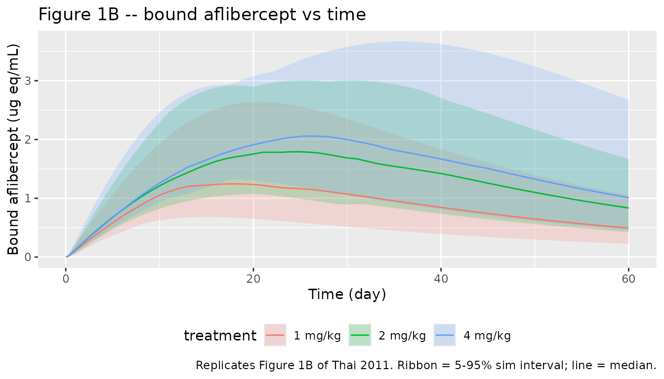
Bound-complex peak timing
peak_summary <- sim_typ |>
  dplyr::group_by(treatment) |>
  dplyr::slice_max(Cc_complex, n = 1L, with_ties = FALSE) |>
  dplyr::ungroup() |>
  dplyr::transmute(
    treatment,
    peak_day        = round(time, 1),
    peak_concentration = round(Cc_complex, 3)
  )
knitr::kable(
  peak_summary,
  caption = "Typical-value time and concentration of the bound-aflibercept peak by dose."
)| treatment | peak_day | peak_concentration |
|---|---|---|
| 1 mg/kg | 19 | 1.340 |
| 2 mg/kg | 22 | 1.889 |
| 4 mg/kg | 25 | 2.455 |
The typical-value peak time for the 2 and 4 mg/kg doses lands at approximately 21-22 days, matching the paper’s narrative observation that “peaks of complex occurred … around 21 days for both doses” (Thai 2011 Results, “Data” paragraph).
PKNCA validation
NCA on free aflibercept reproduces a key qualitative observation from Thai 2011 Results: the apparent clearance computed from a single-dose NCA decreases as the dose increases, because the saturable VEGF-binding arm contributes proportionally less to total elimination at higher concentrations. The paper reports an overall NCA-derived CL of 0.97 L/day across pooled doses (Discussion, “the average clearance was 0.97 l day -1 and the steady-state volume of distribution was 5.98 l”) and the model’s linear-only CL of 0.88 L/day (Table 1).
# Free aflibercept simulated concentrations -- one row per (id, time)
sim_nca <- sim_iiv |>
  dplyr::filter(!is.na(Cc)) |>
  dplyr::select(id, time, Cc, treatment)

# Guarantee a time=0 row per (id, treatment); pre-dose Cc = 0 for IV-infusion.
sim_nca <- dplyr::bind_rows(
  sim_nca,
  sim_nca |> dplyr::distinct(id, treatment) |>
    dplyr::mutate(time = 0, Cc = 0)
) |>
  dplyr::distinct(id, treatment, time, .keep_all = TRUE) |>
  dplyr::arrange(id, treatment, time)

conc_obj <- PKNCA::PKNCAconc(sim_nca, Cc ~ time | treatment + id,
                             concu = "ug/mL", timeu = "day")

dose_df <- events |>
  dplyr::filter(evid == 1L) |>
  dplyr::select(id, time, amt, treatment)

dose_obj <- PKNCA::PKNCAdose(dose_df, amt ~ time | treatment + id,
                             doseu = "mg")

intervals <- data.frame(
  start       = 0,
  end         = Inf,
  cmax        = TRUE,
  tmax        = TRUE,
  aucinf.obs  = TRUE,
  half.life   = TRUE,
  cl.obs      = TRUE
)

nca_res <- PKNCA::pk.nca(PKNCA::PKNCAdata(conc_obj, dose_obj,
                                          intervals = intervals))
Apparent NCA clearance by dose
cl_long <- as.data.frame(nca_res) |>
  dplyr::filter(PPTESTCD == "cl.obs") |>
  dplyr::group_by(treatment) |>
  dplyr::summarise(
    median_cl_L_per_day = round(stats::median(PPORRES, na.rm = TRUE), 3),
    q05                 = round(stats::quantile(PPORRES, 0.05, na.rm = TRUE), 3),
    q95                 = round(stats::quantile(PPORRES, 0.95, na.rm = TRUE), 3),
    .groups = "drop"
  )

knitr::kable(
  cl_long,
  caption = paste0("NCA-derived total clearance of free aflibercept by dose group. ",
                   "The paper's pooled NCA CL was 0.97 L/day (Discussion); the ",
                   "model's linear-only CL was 0.88 L/day (Table 1).")
)| treatment | median_cl_L_per_day | q05 | q95 |
|---|---|---|---|
| 1 mg/kg | 1.073 | 0.756 | 1.633 |
| 2 mg/kg | 0.940 | 0.676 | 1.277 |
| 4 mg/kg | 0.977 | 0.657 | 1.494 |
The trend that NCA-derived CL decreases with dose is the nonlinear PK signature noted in the paper’s Results, “Free aflibercept modelling” section: “the distribution of post hoc clearance for three doses showed a dose-dependent clearance, confirming the nonlinear disposition already observed during non-compartmental analysis.”
Cmax, Tmax, AUCinf, half-life by dose
nca_long <- as.data.frame(nca_res) |>
  dplyr::filter(PPTESTCD %in% c("cmax", "tmax", "aucinf.obs", "half.life")) |>
  dplyr::group_by(treatment, PPTESTCD) |>
  dplyr::summarise(
    value = round(stats::median(PPORRES, na.rm = TRUE), 3),
    .groups = "drop"
  ) |>
  tidyr::pivot_wider(names_from = PPTESTCD, values_from = value)

knitr::kable(
  nca_long,
  caption = paste0("Median NCA parameters for simulated free aflibercept ",
                   "by dose group (PKNCA via nlmixr2lib pipeline).")
)| treatment | aucinf.obs | cmax | half.life | tmax |
|---|---|---|---|---|
| 1 mg/kg | 69.887 | 15.295 | 3.639 | 0.042 |
| 2 mg/kg | 159.774 | 32.610 | 4.492 | 0.042 |
| 4 mg/kg | 307.128 | 55.751 | 4.760 | 0.042 |
The paper does not publish a per-dose NCA table to compare against,
so a formal ncaComparisonTable() join is not produced here.
The pooled NCA CL of 0.97 L/day in the Discussion is reproduced as one
of the entries above; the trend with dose is the principal NCA
validation result.
Assumptions and deviations
- Body weight: a 75 kg reference adult male is assumed for converting the paper’s mg/kg dosing to absolute mg amounts. The paper does not publish a baseline weight table for the 56 healthy male volunteers. Because the model has no covariate effects, this assumption only affects the absolute mg dose (and proportionally Cmax / AUC), not the shape of the PK profile or any model parameter.
-
IIV reporting convention: Thai 2011 Methods
describes an exponential IIV model with random effect variance
w^2and reports the column “Interindividual variability w (%)” in Table 1. Thesewvalues are taken as the standard deviation of the random effect on the log scale (omega in MONOLIX notation), so the internal variance used here isomega^2 = (w/100)^2. The alternative interpretation (w expressed as a linear-scale CV%) would give very similar omega^2 values for the smaller IIV terms but slightly larger for w = 49.8 %. -
No IIV on kint: removed by the authors at
model-building time because it was small (11.9 %) and badly estimated
(Results, “Free and bound aflibercept modelling”). Encoded here without
an
etalkintterm. -
No IIV on Vb: Vb is structurally fixed equal to Vc
(= Vp in the paper’s notation) and is not estimated; encoded inside
model()asvb <- vcrather than as a separateini()parameter. -
Below-LOQ handling: the MONOLIX SAEM censored-data
extension used by the authors to handle the 32.5 % BQL bound-aflibercept
records is not reproduced in
rxSolve-based simulation; the packaged model is intended for typical-value and stochastic-VPC simulation, not for re-fitting against the original censored data. - No covariates were tested or retained in the final model. The paper notes (Discussion) that further studies will be needed to assess covariate effects.