Penciclovir / famciclovir (Ogungbenro 2009)
Source:vignettes/articles/Ogungbenro_2009_penciclovir.Rmd
Ogungbenro_2009_penciclovir.RmdModel and source
- Citation: Ogungbenro K, Matthews I, Looby M, Kaiser G, Graham G, Aarons L. (2009). Population pharmacokinetics and optimal design of paediatric studies for famciclovir. British Journal of Clinical Pharmacology 68(4):546-560. doi:10.1111/j.1365-2125.2009.03479.x
- Description: Two-compartment population PK model with first-order absorption and lag time for penciclovir in pooled adults and children (Ogungbenro 2009). Famciclovir is the oral prodrug of penciclovir; both oral famciclovir and intravenous penciclovir doses are described jointly (six clinical studies, 69 subjects of whom 23 are children, 160 occasions, 1676 plasma penciclovir observations). Allometric body-weight scaling with reference 70 kg (exponent 0.75 shared on CL and Q, exponent 1.0 shared on V1 and V2), an empirical piecewise age effect on CL with separate K parameters for AGE < 40 years (rising-with-youth limb) and AGE >= 40 years (declining-with-elderly limb), and a power function of creatinine clearance on CL with reference 100 mL/min (Cockcroft-Gault, raw mL/min). Inter-individual variability on ka, CL, V1 (fixed at omega^2 = 0.003), V2, and Q; combined proportional plus additive residual error (additive variance fixed at 0.01 mg2/L2).
- Article: https://doi.org/10.1111/j.1365-2125.2009.03479.x
Population
Ogungbenro and colleagues pooled penciclovir plasma concentrations
from six Novartis clinical trials covering 69 subjects (160 occasions,
1676 observations): a single-ascending-dose adult oral study, an adult
IV / oral crossover bioavailability study, a single-oral-dose
renal-impairment study, a single-IV-infusion immunocompromised
paediatric study (2-17 years; two subjects also received an oral washout
dose), a multiple-oral-dose paediatric hepatitis B study (6-11 years),
and a multiple-IV-infusion adult study. The combined cohort spanned 2-63
years and 13.9-94.6 kg; serum creatinine 0.28-1.94 mg/dL;
Cockcroft-Gault creatinine clearance 27.6-175.6 mL/min. Sex was 62 M / 7
F (Tables 1 and 2 of Ogungbenro 2009). The same information is available
programmatically via
readModelDb("Ogungbenro_2009_penciclovir")$population.
Source trace
The per-parameter origin is recorded as an in-file comment next to
each ini() entry in
inst/modeldb/specificDrugs/Ogungbenro_2009_penciclovir.R.
The table below collects them in one place for review.
| Equation / parameter | Value | Source location |
|---|---|---|
ka |
1.86 1/h | Table 4 row ka
|
CL (ref subject) |
31.2 L/h | Table 4 row CL (l h-1 70 kg-1)
|
V1 |
28.6 L | Table 4 row V1 (l.70 kg-1)
|
V2 |
54.5 L | Table 4 row V2 (l.70 kg-1)
|
Q |
60.2 L/h | Table 4 row Q (l h-1 70 kg-1)
|
F |
0.598 | Table 4 row F
|
Tlag |
0.206 h | Table 4 row Tlag (h)
|
| WT exponent on CL, Q | 0.75 (fixed) | Methods, allometric-model paragraph |
| WT exponent on V1, V2 | 1.0 (fixed) | Methods, allometric-model paragraph |
K_AGE for AGE < 40 |
159 years | Table 4 row K_AGE < 40
|
K_AGE for AGE >= 40 |
113 years | Table 4 row K_AGE >= 40
|
| CRCL exponent on CL | 0.28 | Table 4 row Exponent of FCL_CR
|
| BSV(ka) omega^2 | 0.640 | Table 4 row BSV_ka
|
| BSV(CL) omega^2 | 0.230 | Table 4 row BSV_CL
|
| BSV(V1) omega^2 | 0.003 (fixed) | Table 4 row BSV_V1
|
| BSV(V2) omega^2 | 0.255 | Table 4 row BSV_V2
|
| BSV(Q) omega^2 | 0.342 | Table 4 row BSV_Q
|
| Proportional sigma^2 | 0.221 | Table 4 row Proportional error
|
| Additive sigma^2 | 0.01 (fixed) | Table 4 row Additive error (mg l-1)
|
| 2-cmt with depot, lag | n/a | Methods, Results paragraphs (“two-compartment first-order absorption”) |
| CL covariate model | n/a | Table 5 final-model row for CL |
Virtual cohort
Original observed data are not publicly available. The figures below use virtual populations whose covariate distributions match the paper’s reference values (Methods, Paediatric dose adjustment paragraph) and Table 1 demographics. For the paediatric age bands, weight and serum creatinine reference ranges are those Ogungbenro 2009 used to extrapolate simulations:
- 1-2 y: 9.9-12.38 kg, SCr 0.40-0.43 mg/dL
- 2-5 y: 12.38-18.37 kg, SCr 0.43-0.50 mg/dL
- 5-12 y: 18.37-38.30 kg, SCr 0.50-0.65 mg/dL
- Adults: WT 70 kg (SD 12), SCr 0.99 mg/dL (SD 0.2)
Creatinine clearance is derived from age, weight, sex, and serum creatinine via the Cockcroft-Gault equation (same as the source paper) – a fixed sex of male is used for simplicity since the cohort was 62 M / 7 F.
set.seed(20260613)

cockcroft_gault <- function(age_years, weight_kg, scr_mg_dL, female = FALSE) {
  raw <- (140 - age_years) * weight_kg / (72 * scr_mg_dL)
  ifelse(female, raw * 0.85, raw)
}

make_cohort <- function(n, treatment, route, dose_mg_per_kg = NA, dose_mg = NA,
                        age_lo, age_hi, wt_lo, wt_hi, scr_lo, scr_hi,
                        sample_times, id_offset = 0L) {
  subj <- tibble(
    id   = id_offset + seq_len(n),
    AGE  = runif(n, age_lo, age_hi),
    WT   = runif(n, wt_lo,  wt_hi),
    SCR  = runif(n, scr_lo, scr_hi)
  ) |>
    mutate(
      CRCL = cockcroft_gault(AGE, WT, SCR, female = FALSE),
      amt  = if (is.na(dose_mg)) dose_mg_per_kg * WT else dose_mg,
      treatment = treatment,
      route     = route
    )

  dose <- subj |>
    mutate(time = 0, evid = 1L, cmt = ifelse(route == "PO", "depot", "central")) |>
    select(id, time, evid, amt, cmt, AGE, WT, CRCL, treatment, route)

  obs <- subj |>
    select(id, AGE, WT, CRCL, treatment, route) |>
    tidyr::crossing(time = sample_times) |>
    mutate(evid = 0L, amt = 0, cmt = "central") |>
    select(id, time, evid, amt, cmt, AGE, WT, CRCL, treatment, route)

  bind_rows(dose, obs) |> arrange(id, time, desc(evid))
}

obs_times <- c(0, 0.25, 0.5, 0.75, 1, 1.5, 2, 3, 4, 6, 8, 10, 12, 16, 24)

cohorts <- bind_rows(
  make_cohort(
    n = 50, treatment = "Adults 500 mg PO", route = "PO", dose_mg = 500,
    age_lo = 25, age_hi = 55, wt_lo = 60, wt_hi = 90,
    scr_lo = 0.79, scr_hi = 1.19, sample_times = obs_times, id_offset = 0L
  ),
  make_cohort(
    n = 50, treatment = "Adults 500 mg IV", route = "IV", dose_mg = 500,
    age_lo = 25, age_hi = 55, wt_lo = 60, wt_hi = 90,
    scr_lo = 0.79, scr_hi = 1.19, sample_times = obs_times, id_offset = 50L
  ),
  make_cohort(
    n = 50, treatment = "Children 1-2 y, 10 mg/kg PO", route = "PO",
    dose_mg_per_kg = 10,
    age_lo = 1, age_hi = 2, wt_lo = 9.9, wt_hi = 12.38,
    scr_lo = 0.40, scr_hi = 0.43, sample_times = obs_times, id_offset = 100L
  ),
  make_cohort(
    n = 50, treatment = "Children 2-5 y, 10 mg/kg PO", route = "PO",
    dose_mg_per_kg = 10,
    age_lo = 2, age_hi = 5, wt_lo = 12.38, wt_hi = 18.37,
    scr_lo = 0.43, scr_hi = 0.50, sample_times = obs_times, id_offset = 150L
  ),
  make_cohort(
    n = 50, treatment = "Children 5-12 y, 10 mg/kg PO", route = "PO",
    dose_mg_per_kg = 10,
    age_lo = 5, age_hi = 12, wt_lo = 18.37, wt_hi = 38.30,
    scr_lo = 0.50, scr_hi = 0.65, sample_times = obs_times, id_offset = 200L
  )
)

stopifnot(!anyDuplicated(unique(cohorts[, c("id", "time", "evid")])))
Simulation
mod <- rxode2::rxode2(readModelDb("Ogungbenro_2009_penciclovir"))
#> ℹ parameter labels from comments will be replaced by 'label()'

sim <- rxode2::rxSolve(
  mod,
  events = cohorts,
  keep   = c("treatment", "route", "WT", "AGE", "CRCL")
) |>
  as.data.frame() |>
  filter(time > 0 | (time == 0 & Cc >= 0))
Replicate published figures
Figure 7 of Ogungbenro 2009 overlays plasma penciclovir 95% prediction intervals and median lines for the three paediatric age groups (10 mg/kg PO) against the 500 mg adult PO reference. The plot below uses the same simulation cohorts to reproduce that overlay shape.
# Replicates Figure 7 of Ogungbenro 2009: 95% prediction intervals and
# median plasma penciclovir for 10 mg/kg PO in three paediatric age groups
# vs 500 mg PO in adults.
sim_po <- sim |>
  filter(route == "PO")

summary_po <- sim_po |>
  group_by(treatment, time) |>
  summarise(
    Q025 = quantile(Cc, 0.025, na.rm = TRUE),
    Q50  = quantile(Cc, 0.50,  na.rm = TRUE),
    Q975 = quantile(Cc, 0.975, na.rm = TRUE),
    .groups = "drop"
  )

ggplot(summary_po, aes(time, Q50, colour = treatment, fill = treatment)) +
  geom_ribbon(aes(ymin = Q025, ymax = Q975), alpha = 0.15, colour = NA) +
  geom_line(linewidth = 0.8) +
  scale_y_continuous(trans = "log10",
                     limits = c(0.01, NA)) +
  labs(x = "Time (h)", y = "Plasma penciclovir (mg/L)",
       title = "Replicates Figure 7: PO penciclovir profiles",
       caption = paste("Adults 500 mg PO vs three paediatric age bands at 10 mg/kg PO;",
                       "median and 95% prediction interval per virtual cohort."),
       colour = "Cohort", fill = "Cohort") +
  theme_minimal()
#> Warning in scale_y_continuous(trans = "log10", limits = c(0.01, NA)): log-10 transformation introduced infinite values.
#> log-10 transformation introduced infinite values.
#> log-10 transformation introduced infinite values.
#> log-10 transformation introduced infinite values.
#> Warning: Removed 21 rows containing missing values or values outside the scale range
#> (`geom_ribbon()`).
#> Warning: Removed 7 rows containing missing values or values outside the scale range
#> (`geom_line()`).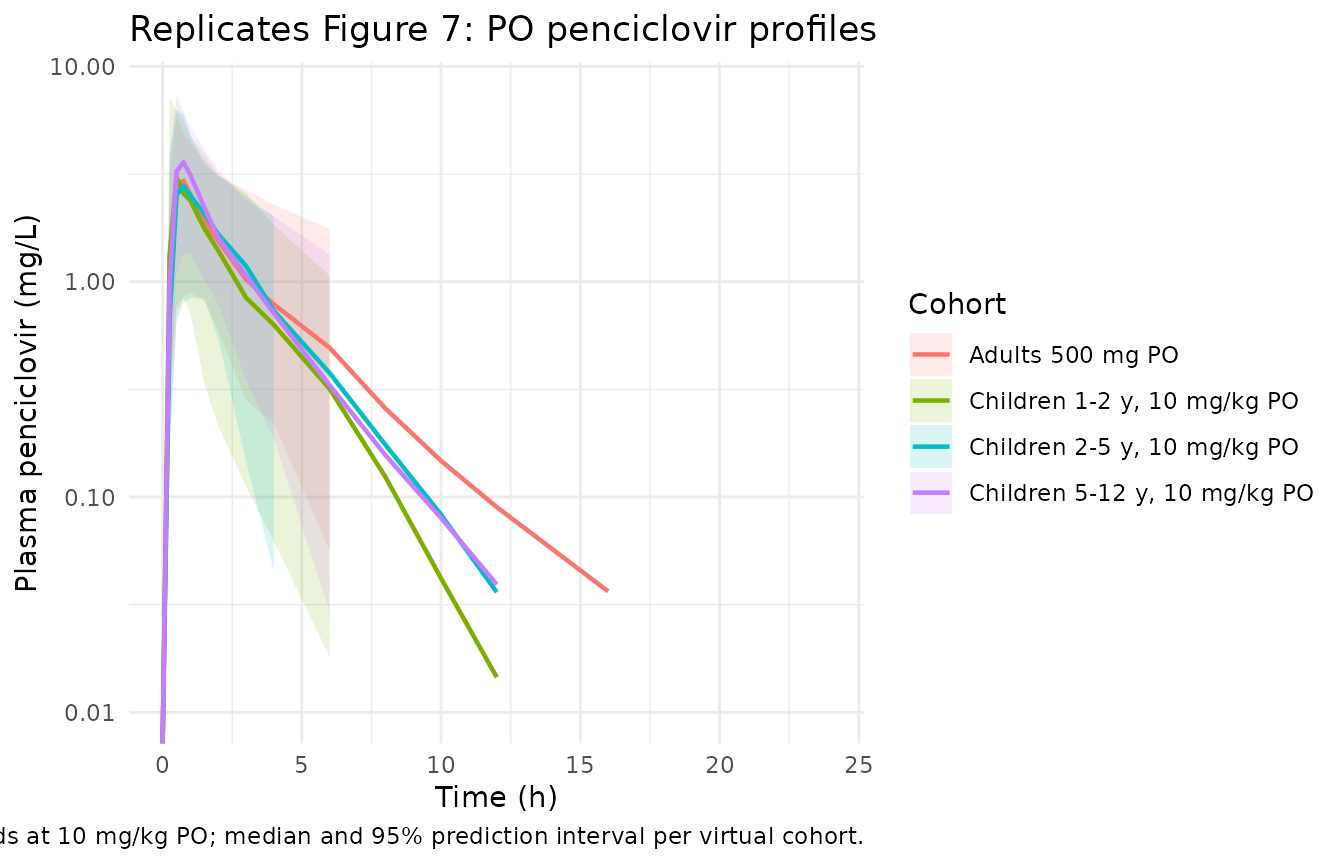
Figure 5 of Ogungbenro 2009 shows a visual predictive check for the pooled adult+paediatric data split by oral and IV routes. The plot below builds the typical-value (zero random-effects) trajectory for the adult 500 mg PO and IV cohorts so the route-specific shapes can be compared at a glance.
mod_typical <- rxode2::zeroRe(mod)
sim_typical <- rxode2::rxSolve(
  mod_typical,
  events = cohorts |> filter(treatment %in% c("Adults 500 mg PO",
                                              "Adults 500 mg IV")),
  keep   = c("treatment", "route", "WT", "AGE", "CRCL")
) |>
  as.data.frame() |>
  filter(time >= 0)
#> ℹ omega/sigma items treated as zero: 'etalka', 'etalcl', 'etalvc', 'etalvp', 'etalq'
#> Warning: multi-subject simulation without without 'omega'

ggplot(sim_typical |>
         group_by(treatment, time) |>
         summarise(Cc = median(Cc, na.rm = TRUE), .groups = "drop"),
       aes(time, Cc, colour = treatment)) +
  geom_line(linewidth = 0.9) +
  scale_y_continuous(trans = "log10", limits = c(0.01, NA)) +
  labs(x = "Time (h)", y = "Plasma penciclovir (mg/L)",
       title = "Typical-value adult profiles: 500 mg PO vs IV",
       caption = "Random-effects zeroed via rxode2::zeroRe().",
       colour = "Cohort") +
  theme_minimal()
#> Warning in scale_y_continuous(trans = "log10", limits = c(0.01, NA)): log-10
#> transformation introduced infinite values.
#> Warning: Removed 2 rows containing missing values or values outside the scale range
#> (`geom_line()`).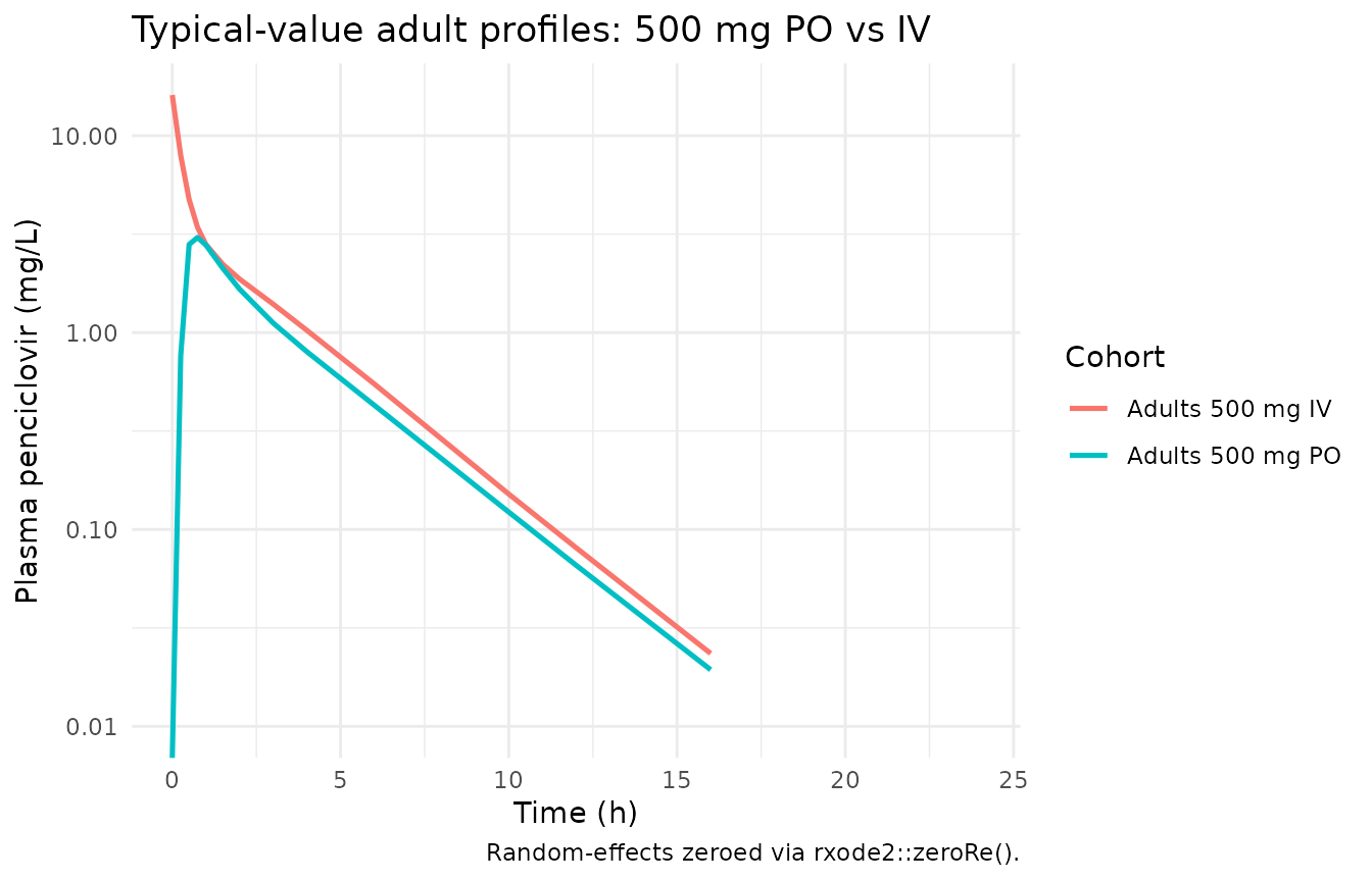
PKNCA validation
sim_nca <- sim |>
  filter(!is.na(Cc)) |>
  select(id, time, Cc, treatment)

# Guarantee a t = 0 row per (id, treatment); pre-dose Cc = 0 is the correct
# value for extravascular dosing and a good back-extrapolation anchor for
# the IV cohort (PKNCA can recompute via lambda.z if needed).
sim_nca <- bind_rows(
  sim_nca,
  sim_nca |> distinct(id, treatment) |> mutate(time = 0, Cc = 0)
) |>
  distinct(id, treatment, time, .keep_all = TRUE) |>
  arrange(id, treatment, time)

conc_obj <- PKNCA::PKNCAconc(
  sim_nca, Cc ~ time | treatment + id,
  concu = "mg/L", timeu = "h"
)
#> Warning in assert_conc(conc, any_missing_conc = any_missing_conc): Negative
#> concentrations found

dose_df <- cohorts |>
  filter(evid == 1) |>
  select(id, time, amt, treatment)

dose_obj <- PKNCA::PKNCAdose(
  dose_df, amt ~ time | treatment + id,
  doseu = "mg"
)

intervals <- data.frame(
  start       = 0,
  end         = Inf,
  cmax        = TRUE,
  tmax        = TRUE,
  aucinf.obs  = TRUE,
  auclast     = TRUE,
  half.life   = TRUE
)

nca_data <- PKNCA::PKNCAdata(conc_obj, dose_obj, intervals = intervals)
nca_res  <- PKNCA::pk.nca(nca_data)
#> Warning in assert_conc(conc, any_missing_conc = any_missing_conc): Negative
#> concentrations found
#> Warning in log(conc.2/conc.1): NaNs produced
#> Warning in assert_conc(conc = conc): Negative concentrations found
#> Warning in assert_conc(conc, any_missing_conc = any_missing_conc): Negative
#> concentrations found
#> Warning in assert_conc(conc, any_missing_conc = any_missing_conc): Negative
#> concentrations found
#> Warning in assert_conc(conc, any_missing_conc = any_missing_conc): Negative
#> concentrations found
#> Warning in assert_conc(conc, any_missing_conc = any_missing_conc): Negative
#> concentrations found
#> Warning in assert_conc(conc, any_missing_conc = any_missing_conc): Negative
#> concentrations found
#> Warning in log(data$conc): NaNs produced
#> Warning in assert_conc(conc, any_missing_conc = any_missing_conc): Negative
#> concentrations found
#> Warning in log(conc.2/conc.1): NaNs produced
#> Warning in assert_conc(conc, any_missing_conc = any_missing_conc): Negative
#> concentrations found
#> Warning in log(conc.2/conc.1): NaNs produced
#> Warning in assert_conc(conc = conc): Negative concentrations found
#> Warning in assert_conc(conc, any_missing_conc = any_missing_conc): Negative
#> concentrations found
#> Warning in assert_conc(conc, any_missing_conc = any_missing_conc): Negative
#> concentrations found
#> Warning in assert_conc(conc, any_missing_conc = any_missing_conc): Negative
#> concentrations found
#> Warning in assert_conc(conc, any_missing_conc = any_missing_conc): Negative
#> concentrations found
#> Warning in assert_conc(conc, any_missing_conc = any_missing_conc): Negative
#> concentrations found
#> Warning in log(data$conc): NaNs produced
#> Warning in assert_conc(conc, any_missing_conc = any_missing_conc): Negative
#> concentrations found
#> Warning in log(conc.2/conc.1): NaNs produced
Comparison against published expectations
The paper does not tabulate cohort-level NCA Cmax / Tmax / AUC for penciclovir directly. Two validation targets are available from the paper text and from the literature it cites:
The Discussion paragraph quantifying model performance: “the mean predicted penciclovir clearance … for adults were 36 l h-1 and 85 l [Vss], respectively, … the adults’ mean clearance and mean total volume of distribution values for penciclovir compare favourably with those obtained from previous noncompartmental analysis, i.e. 36.6 +/- 6.3 l h-1 and 1.08 +/- 0.17 l kg-1.” For the 500 mg PO adult cohort, apparent clearance from PKNCA
CL/F = dose / AUC0-infshould approach36 / 0.598 ~= 60 L/hin the deterministic limit; this is reported next to the published value.The Results paragraph quantifying the 10 mg/kg paediatric dose selection: “[10 mg/kg] gave an AUC ratio (paediatric mean/adult mean) that is close to 1 (0.95, 0.96, 1.02 for the three paediatric age groups), while the Cmax ratio is < 1.2 (1.05, 1.10 and 1.15 for the three paediatric age groups).” These six ratios are direct validation targets for the paediatric / adult PO simulations and are tabulated below.
res_tbl <- as.data.frame(nca_res$result)

# Median per (treatment, parameter)
nca_summary <- res_tbl |>
  group_by(treatment, PPTESTCD) |>
  summarise(value = median(PPORRES, na.rm = TRUE), .groups = "drop") |>
  pivot_wider(names_from = PPTESTCD, values_from = value)

nca_summary |>
  select(treatment, cmax, tmax, auclast, aucinf.obs, half.life) |>
  mutate(across(c(cmax, tmax, auclast, aucinf.obs, half.life),
                ~ signif(.x, 3))) |>
  dplyr::rename(
    "Cohort"              = treatment,
    "Cmax (mg/L)"         = cmax,
    "Tmax (h)"            = tmax,
    "AUClast (mg*h/L)"    = auclast,
    "AUCinf,obs (mg*h/L)" = aucinf.obs,
    "t1/2 (h)"            = half.life
  ) |>
  knitr::kable(
    caption = "Per-cohort median PKNCA-derived parameters."
)| Cohort | Cmax (mg/L) | Tmax (h) | AUClast (mg*h/L) | AUCinf,obs (mg*h/L) | t1/2 (h) |
|---|---|---|---|---|---|
| Adults 500 mg IV | 16.50 | 0.00 | 13.00 | 13.00 | 2.65 |
| Adults 500 mg PO | 3.21 | 0.75 | 9.36 | 9.40 | 2.91 |
| Children 1-2 y, 10 mg/kg PO | 3.24 | 0.50 | 8.38 | 8.38 | 1.65 |
| Children 2-5 y, 10 mg/kg PO | 2.87 | 0.75 | 9.68 | 9.72 | 1.84 |
| Children 5-12 y, 10 mg/kg PO | 3.67 | 0.75 | 9.33 | 9.34 | 1.86 |
# Paediatric / adult ratios for AUC and Cmax (the paper's Results targets).
adult_po <- nca_summary |> filter(treatment == "Adults 500 mg PO")

ratio_tbl <- nca_summary |>
  filter(grepl("^Children", treatment)) |>
  mutate(
    auc_ratio_sim  = aucinf.obs / adult_po$aucinf.obs,
    cmax_ratio_sim = cmax       / adult_po$cmax
  ) |>
  select(treatment, auc_ratio_sim, cmax_ratio_sim)

# Paper's reported ratios (Results, Paediatric dose adjustment paragraph).
published_ratios <- tibble::tribble(
  ~treatment,                       ~auc_ratio_paper, ~cmax_ratio_paper,
  "Children 1-2 y, 10 mg/kg PO",    0.95,             1.05,
  "Children 2-5 y, 10 mg/kg PO",    0.96,             1.10,
  "Children 5-12 y, 10 mg/kg PO",   1.02,             1.15
)

compare_tbl <- ratio_tbl |>
  left_join(published_ratios, by = "treatment") |>
  mutate(
    auc_pct_diff  = 100 * (auc_ratio_sim  - auc_ratio_paper)  / auc_ratio_paper,
    cmax_pct_diff = 100 * (cmax_ratio_sim - cmax_ratio_paper) / cmax_ratio_paper
  ) |>
  mutate(across(c(auc_ratio_sim, auc_ratio_paper, cmax_ratio_sim, cmax_ratio_paper),
                ~ signif(.x, 3)),
         across(c(auc_pct_diff, cmax_pct_diff), ~ round(.x, 1)))

compare_tbl |>
  dplyr::rename(
    "Cohort"            = treatment,
    "AUC ratio (sim)"   = auc_ratio_sim,
    "Cmax ratio (sim)"  = cmax_ratio_sim,
    "AUC ratio (paper)" = auc_ratio_paper,
    "Cmax ratio (paper)" = cmax_ratio_paper,
    "AUC % diff"        = auc_pct_diff,
    "Cmax % diff"       = cmax_pct_diff
  ) |>
  knitr::kable(
    caption = paste("Paediatric / adult exposure ratios at 10 mg/kg PO,",
                    "simulated vs Ogungbenro 2009 Results section.")
)| Cohort | AUC ratio (sim) | Cmax ratio (sim) | AUC ratio (paper) | Cmax ratio (paper) | AUC % diff | Cmax % diff |
|---|---|---|---|---|---|---|
| Children 1-2 y, 10 mg/kg PO | 0.892 | 1.010 | 0.95 | 1.05 | -6.1 | -4.0 |
| Children 2-5 y, 10 mg/kg PO | 1.030 | 0.895 | 0.96 | 1.10 | 7.8 | -18.6 |
| Children 5-12 y, 10 mg/kg PO | 0.994 | 1.140 | 1.02 | 1.15 | -2.6 | -0.7 |
# Adult apparent clearance from PO PKNCA: CL/F = dose / AUCinf.
adult_clf <- 500 / adult_po$aucinf.obs
adult_cl  <- adult_clf * 0.598

clearance_tbl <- tibble::tribble(
  ~Metric,                                              ~Value,
  "Adult typical CL/F (sim, mg / (mg*h/L) = L/h)",      as.character(signif(adult_clf, 3)),
  "Adult typical CL  (sim, L/h)",                       as.character(signif(adult_cl, 3)),
  "Paper-reported mean predicted CL (L/h)",             "36",
  "Literature noncompartmental CL (L/h)",               "36.6 +/- 6.3"
)

knitr::kable(
  clearance_tbl,
  caption = paste("Adult 500 mg PO apparent and absolute clearance,",
                  "simulated vs Ogungbenro 2009 Discussion values.")
)| Metric | Value |
|---|---|
| Adult typical CL/F (sim, mg / (mg*h/L) = L/h) | 53.2 |
| Adult typical CL (sim, L/h) | 31.8 |
| Paper-reported mean predicted CL (L/h) | 36 |
| Literature noncompartmental CL (L/h) | 36.6 +/- 6.3 |
Assumptions and deviations
-
Sex distribution. Cockcroft-Gault creatinine
clearance was computed for an all-male virtual cohort. The pooled study
population was 62 M / 7 F (90% male; Table 2); sex was not retained in
the final model, so a uniform-male assumption affects only the CRCL
input distribution, not the structural model. With female multiplier
0.85, a female of the same age and weight would have ~15% lower CRCL and
~4% lower CL via
(CRCL/100)^0.28. - Sample times. A common observation grid (0, 0.25, 0.5, 0.75, 1, 1.5, 2, 3, 4, 6, 8, 10, 12, 16, 24 h) was applied across all cohorts to support a single PKNCA call. The paper’s optimised sampling-windows design (Table 6) is itself a methodology output of the paper, not an input to the PK model, and is therefore not reproduced here.
- Race / ethnicity. Not reported in the source paper. No race covariate appears in the model.
- Creatinine clearance. Computed via Cockcroft-Gault (raw mL/min) on the virtual cohort, matching the source paper’s covariate assay. Per the covariate-columns register, the canonical CRCL column accepts raw Cockcroft-Gault mL/min when the per-model description records the assay form – this model records it as such.
- Reference dose for the comparison ratio. The paper computes AUC and Cmax ratios against an adult reference of 500 mg PO famciclovir. The virtual adult cohort uses the same 500 mg PO single-dose regimen.
- Half-life from PKNCA. PKNCA computes terminal half-life from the log-linear regression of the post-Cmax decline; the two-compartment structural model produces a biphasic decline whose effective terminal slope depends on the observation window. The reported t1/2 values are apparent post-Cmax terminal half-lives from the 0-24 h window.