Oxcarbazepine (Jang 2021) • nlmixr2lib

Model and source

Citation: Jang Y, Yoon S, Kim TJ, Lee S, Yu KS, Jang IJ, Chu K, Lee SK. Population pharmacokinetic model development and its relationship with adverse events of oxcarbazepine in adult patients with epilepsy. Sci Rep. 2021;11:6370. doi:10.1038/s41598-021-85920-0
Description: One-compartment population PK model with first-order absorption and elimination for the monohydroxy derivative (MHD, licarbazepine) of oral oxcarbazepine in Korean adults with epilepsy (Jang 2021). Oxcarbazepine doses drive MHD directly (parent not modelled); apparent clearance CL/F and apparent volume V/F scale with body weight by estimated power exponents centred at 66 kg. Inter-individual variability on CL/F and on the absorption rate constant ka (the control stream fixes the V/F variance to zero), with a proportional residual error.
Article: https://doi.org/10.1038/s41598-021-85920-0 (open access)
Supplementary material: the NONMEM control stream of the final model (41598_2021_85920_MOESM2_ESM.docx) and the goodness-of-fit figure plus co-medication table (41598_2021_85920_MOESM1_ESM.docx), both linked from the article page.

Jang 2021 built the population PK model to convert sparse spot concentrations of the active monohydroxy derivative (MHD, licarbazepine) into individual exposure metrics – a steady-state trough and AUC = Dose / (CL/F) – and then related those metrics to dose-related adverse events (dizziness, somnolence, headache, diplopia). The PK model is the part extracted here. Oxcarbazepine itself is not modelled: its exposure is about 1/15 of MHD’s, so each oxcarbazepine dose (mg) enters the depot and the central compartment holds MHD in oxcarbazepine-mg equivalents (the molar masses are 252.3 and 254.3 g/mol, so the two scales agree to within 1%).

Population

The PK dataset combined two sources (Jang 2021 Methods):

Study 1, the Epilepsy Registry Cohort of Seoul National University Hospital (February 2011 to January 2014): single spot samples from adults on an unchanged oxcarbazepine dose for at least one month, assumed to be at steady state. Of 618 patients with 711 samples, 447 had complete body-weight, last-dose and sampling-time records. 438 took oxcarbazepine twice daily, 5 once daily and 4 three times daily.
Study 2, a single-dose oral-loading study in 40 patients with epilepsy (30 mg/kg; Kim DW et al. Epilepsia 2012;53:e9-12), sampled at 2, 4, 6, 8, 12, 14, 16 and 24 h.

In total 748 MHD concentrations from 487 patients were modelled. Table 1 and the Results describe the 447 registry patients: 59.1% male, mean age 39.2 years (range 16-80), mean body weight 65.8 kg (range 39-116), mean daily dose 999 mg (range 150-2100 mg/day), 65.3% on at least one other antiseizure medication (most often levetiracetam, 55.5%, and topiramate, 32.9%) and 5.1% on an enzyme-inducing one. All patients were Korean.

str(readModelDb("Jang_2021_oxcarbazepine")()$population)
#> List of 14
#>  $ species       : chr "human"
#>  $ n_subjects    : int 487
#>  $ n_studies     : int 2
#>  $ n_observations: int 748
#>  $ age_range     : chr "16-80 years (registry cohort)"
#>  $ age_mean      : chr "39.2 +/- 14.7 years (registry cohort)"
#>  $ weight_range  : chr "39-116 kg (registry cohort)"
#>  $ weight_mean   : chr "65.8 +/- 12.5 kg (registry cohort)"
#>  $ sex_female_pct: num 40.9
#>  $ race_ethnicity: Named num 100
#>   ..- attr(*, "names")= chr "Korean"
#>  $ disease_state : chr "Adults with epilepsy on chronic oxcarbazepine therapy (Study 1, Epilepsy Registry Cohort; 65.3% on at least one"| __truncated__
#>  $ dose_range    : chr "Study 1: stable oral oxcarbazepine for at least one month, mean 999 mg/day (range 150-2100 mg/day), 438 of 447 "| __truncated__
#>  $ regions       : chr "South Korea (Seoul National University Hospital)"
#>  $ notes         : chr "The PK dataset held 748 MHD concentrations from 487 patients (Jang 2021 Methods): the 447 registry patients wit"| __truncated__

Source trace

Every ini() entry in inst/modeldb/specificDrugs/Jang_2021_oxcarbazepine.R carries an in-file comment naming its source. The final estimates come from Jang 2021 Table 2; the model structure comes from the supplementary NONMEM control stream, whose $THETA / $OMEGA records are initial estimates and are not used as values.

Equation / parameter	Value	Source location
One compartment, first-order absorption (`ADVAN2 TRANS2`)	n/a	Methods, Population PK model development; supplementary code `$SUBROUTINE`
`CL/F = theta1 * exp(eta1) * (WT/66)^theta2`	n/a	Table 2 structural block; supplementary code `CL = TVCLEXP(ETA(1))(BW/66)**THETA(4)`
`V/F = theta3 * (WT/66)^theta4`	n/a	Table 2 structural block; supplementary code `V = TVVEXP(ETA(2))(BW/66)**THETA(5)` with `$OMEGA 0 FIX` for `ETA(2)`
`ka = theta * exp(eta3)`	n/a	supplementary code `KA = TVKA*EXP(ETA(3))`
`lcl` (CL/F at 66 kg)	1.65 L/h (1.8% RSE)	Table 2 theta1; bootstrap 1.65 (1.59-1.70)
`e_wt_cl`	0.67 (14.2% RSE)	Table 2 theta2; bootstrap 0.66 (0.47-0.85)
`lvc` (V/F at 66 kg)	59.0 L (4.5% RSE)	Table 2 theta3 (unit printed as L/h, a typo for L); bootstrap 59.2 (54.2-64.8)
`e_wt_vc`	0.96 (18.1% RSE)	Table 2 theta4; bootstrap 0.95 (0.59-1.3)
`lka`	0.34 1/h (9.7% RSE)	Table 2 ka; bootstrap 0.34 (0.28-0.41)
`etalcl`	29.2 %CV -> `omega^2 = log(1 + 0.292^2) = 0.08183`	Table 2 ‘IIV CL/F’
`etalka`	41.5 %CV -> `omega^2 = log(1 + 0.415^2) = 0.15952`	Table 2 second IIV row (labelled ‘IIV V2/F’); assigned to ka per the control stream, see below
`propSd`	0.13	Table 2 ‘Proportional error (SD)’; supplementary code `W = SQRT(THETA(6)2 + THETA(7)2IPRED*2)` with `$SIGMA 1 FIX`
Additive error `THETA(6)`	0.0001 ng/mL, fixed	supplementary code; omitted (see Assumptions)

Which parameter carries the second IIV?

Table 2 labels its second inter-individual variability “IIV V2/F” (41.5 %CV), but the supplementary control stream – captioned “NONMEM code for the final model” – fixes the variance of ETA(2) on V to zero and estimates ETA(3) on KA. Both sources list exactly two estimated variances, so the question is only which parameter the 41.5 %CV belongs to.

Figure 1 (right panel, Study 2) settles it. For a single mg/kg dose the body-weight terms nearly cancel, so the width of the simulated 5th-95th percentile band around the peak is set by the IIV: 41.5 %CV on V/F scales the whole curve and gives a wide band, while 41.5 %CV on ka mostly shifts the rise. The maintainers digitised the simulated percentile bands of Figure 1 (centre of each shaded band) and compared them with both readings, using the closed-form one-compartment solution and base-R draws so the comparison is identical on every machine.

# Figure 1, Study 2: centres of the simulated percentile bands digitised from
# the published raster (time in h, concentration in mg/L).
fig1 <- tibble::tribble(
  ~time, ~p05, ~p50, ~p95,
  6,     18.1, 24.8, 32.8,
  12,    18.3, 24.2, 30.0,
  20,    12.9, 19.3, 26.0
)

closed_form <- function(time, dose, cl, v, ka) {
  k <- cl / v
  dose / v * ka / (ka - k) * (exp(-k * time) - exp(-ka * time))
}

set.seed(20210318)
n_draw <- 2000
wt <- numeric(0)
while (length(wt) < n_draw) {
  x <- rnorm(n_draw, 65.8, 12.5)
  wt <- c(wt, x[x >= 39 & x <= 116])
}
wt <- wt[seq_len(n_draw)]
eta_cl <- rnorm(n_draw, 0, sqrt(log(1 + 0.292^2)))
eta_2 <- rnorm(n_draw, 0, sqrt(log(1 + 0.415^2)))
eps <- rnorm(n_draw, 0, 0.13)

band <- function(eta_v, eta_ka) {
  bind_rows(lapply(fig1$time, function(tm) {
    conc <- closed_form(
      tm,
      dose = 30 * wt,
      cl = 1.65 * exp(eta_cl) * (wt / 66)^0.67,
      v = 59.0 * exp(eta_v) * (wt / 66)^0.96,
      ka = 0.34 * exp(eta_ka)
    ) * (1 + eps)
    tibble(
      time = tm,
      p05 = quantile(conc, 0.05, names = FALSE),
      p50 = quantile(conc, 0.50, names = FALSE),
      p95 = quantile(conc, 0.95, names = FALSE)
    )
  }))
}

hyp <- bind_rows(
  band(eta_v = 0, eta_ka = eta_2) |> mutate(reading = "IIV on ka (control stream)"),
  band(eta_v = eta_2, eta_ka = 0) |> mutate(reading = "IIV on V/F (Table 2 label)")
) |>
  left_join(fig1, by = "time", suffix = c("", "_fig"))

hyp |>
  transmute(
    Reading = reading, `Time (h)` = time,
    `5th` = round(p05, 1), `5th, Fig. 1` = p05_fig,
    `50th` = round(p50, 1), `50th, Fig. 1` = p50_fig,
    `95th` = round(p95, 1), `95th, Fig. 1` = p95_fig
  ) |>
  knitr::kable(caption = paste(
    "Simulated percentiles (mg/L) after a single 30 mg/kg dose under the two",
    "readings of the second IIV, against the Figure 1 simulated bands."
  ))

Simulated percentiles (mg/L) after a single 30 mg/kg dose under the two readings of the second IIV, against the Figure 1 simulated bands.
Reading	Time (h)	5th	5th, Fig. 1	50th	50th, Fig. 1	95th	95th, Fig. 1
IIV on ka (control stream)	6	17.8	18.1	25.4	24.8	32.8	32.8
IIV on ka (control stream)	12	18.5	18.3	25.0	24.2	31.3	30.0
IIV on ka (control stream)	20	14.2	12.9	20.7	19.3	27.2	26.0
IIV on V/F (Table 2 label)	6	13.7	18.1	26.0	24.8	47.5	32.8
IIV on V/F (Table 2 label)	12	14.0	18.3	24.7	24.2	41.9	30.0
IIV on V/F (Table 2 label)	20	11.9	12.9	19.6	19.3	31.7	26.0


ka_reading <- filter(hyp, reading == "IIV on ka (control stream)")
v_reading <- filter(hyp, reading == "IIV on V/F (Table 2 label)")
# The control-stream reading reproduces every Figure 1 band within 15%.
stopifnot(
  all(abs(ka_reading$p05 / ka_reading$p05_fig - 1) < 0.15),
  all(abs(ka_reading$p50 / ka_reading$p50_fig - 1) < 0.15),
  all(abs(ka_reading$p95 / ka_reading$p95_fig - 1) < 0.15)
)
# The Table 2-label reading puts the 6 h 95th percentile far above the
# published band (about 47 vs 33 mg/L).
stopifnot(v_reading$p95[v_reading$time == 6] > 1.25 * 32.8)

The control-stream reading reproduces the published bands; the other reading puts the 6 h 95th percentile about 45% above the figure. The model therefore places the 41.5 %CV on ka, and the “V2/F” label in Table 2 is treated as a typographical error.

Typical-value identity

At the 66 kg reference weight, with random effects removed, the packaged model must reproduce the closed-form one-compartment solution with the Table 2 estimates.

mod <- readModelDb("Jang_2021_oxcarbazepine")
mod_typ <- rxode2::zeroRe(mod)
#> ℹ parameter labels from comments will be replaced by 'label()'

typ_ev <- bind_rows(
  tibble(id = 1L, time = 0, evid = 1L, amt = 30 * 66, cmt = "depot"),
  tibble(id = 1L, time = c(0, 1, 2, 4, 6, 8, 12, 16, 24, 48), evid = 0L,
         amt = 0, cmt = "central")
) |>
  mutate(WT = 66)

typ <- rxode2::rxSolve(mod_typ, typ_ev, returnType = "data.frame",
                       atol = 1e-10, rtol = 1e-10)
#> ℹ omega/sigma items treated as zero: 'etalcl', 'etalka'
expected <- closed_form(typ$time, dose = 30 * 66, cl = 1.65, v = 59.0, ka = 0.34)
stopifnot(
  all(abs(typ$cl - 1.65) < 1e-10),
  all(abs(typ$vc - 59.0) < 1e-10),
  all(abs(typ$Cc - expected) <= 1e-6 * max(expected))
)
knitr::kable(
  tibble(`Time (h)` = typ$time, `Model Cc (mg/L)` = signif(typ$Cc, 5),
         `Closed form (mg/L)` = signif(expected, 5)),
  caption = "Typical 66 kg patient, single 30 mg/kg dose."
)

Typical 66 kg patient, single 30 mg/kg dose.
Time (h)	Model Cc (mg/L)	Closed form (mg/L)
0	0.0000	0.0000
1	9.5312	9.5312
2	16.0520	16.0520
4	23.3120	23.3120
6	26.1640	26.1640
8	26.8280	26.8280
12	25.5240	25.5240
16	23.2170	23.2170
24	18.6790	18.6790
48	9.5522	9.5522

Virtual cohort

Two cohorts of 200 virtual patients each, with body weight drawn from the registry distribution (mean 65.8 kg, SD 12.5 kg, redrawn outside the observed 39-116 kg range):

Single dose – 30 mg/kg once, as in Study 2.
Steady state – twice-daily dosing at a total daily dose drawn from the registry distribution (mean 999 mg/day, SD 338 mg/day, redrawn outside the observed 150-2100 mg/day range), as in Study 1.

draw_in_range <- function(n, mean, sd, lower, upper) {
  out <- numeric(0)
  while (length(out) < n) {
    x <- rnorm(n, mean, sd)
    out <- c(out, x[x >= lower & x <= upper])
  }
  out[seq_len(n)]
}

set.seed(6370)
n_sub <- 200
sd_subj <- tibble(id = seq_len(n_sub),
                  WT = draw_in_range(n_sub, 65.8, 12.5, 39, 116),
                  treatment = "30 mg/kg single dose")
ss_subj <- tibble(id = n_sub + seq_len(n_sub),
                  WT = draw_in_range(n_sub, 65.8, 12.5, 39, 116),
                  daily_dose = draw_in_range(n_sub, 999, 338, 150, 2100),
                  treatment = "Twice daily, steady state")

obs_sd <- c(0, 0.5, 1, 1.5, 2, 3, 4, 5, 6, 7, 8, 10, 12, 14, 16, 18, 20, 22, 24)
sd_ev <- bind_rows(
  sd_subj |> mutate(time = 0, evid = 1L, amt = 30 * WT, ii = 0, ss = 0L,
                    cmt = "depot"),
  sd_subj |> tidyr::crossing(time = obs_sd) |>
    mutate(evid = 0L, amt = 0, ii = 0, ss = 0L, cmt = "central")
)
# ss = 1 at time 0 puts the subject at steady state; addl = 1 gives the
# second dose of the 24 h window.
ss_ev <- bind_rows(
  ss_subj |> mutate(time = 0, evid = 1L, amt = daily_dose / 2, ii = 12,
                    ss = 1L, addl = 1L, cmt = "depot"),
  ss_subj |> tidyr::crossing(time = seq(0, 24, by = 0.5)) |>
    mutate(evid = 0L, amt = 0, ii = 0, ss = 0L, addl = 0L, cmt = "central")
)
events <- bind_rows(sd_ev, ss_ev) |>
  mutate(addl = coalesce(addl, 0L)) |>
  select(id, time, evid, amt, ii, ss, addl, cmt, WT, treatment) |>
  arrange(id, time, desc(evid))
stopifnot(!anyDuplicated(unique(events[, c("id", "time", "evid")])))

Simulation

rxode2::rxSetSeed(6370)
# steady-state searches for long-half-life subjects exceed the default step budget
sim <- rxode2::rxSolve(mod, events, keep = "treatment",
                       returnType = "data.frame", maxsteps = 1e6) |>
  filter(!is.na(Cc))
#> ℹ parameter labels from comments will be replaced by 'label()'

Replicating Figure 1, Study 2

vpc <- sim |>
  filter(treatment == "30 mg/kg single dose") |>
  group_by(time) |>
  summarise(p05 = quantile(sim, 0.05), p50 = quantile(sim, 0.50),
            p95 = quantile(sim, 0.95), .groups = "drop")

fig1_long <- fig1 |>
  pivot_longer(-time, names_to = "percentile", values_to = "conc")

ggplot(vpc, aes(time)) +
  geom_ribbon(aes(ymin = p05, ymax = p95), fill = "steelblue", alpha = 0.25) +
  geom_line(aes(y = p50), colour = "steelblue4", linewidth = 1) +
  geom_point(data = fig1_long, aes(y = conc, shape = percentile), size = 2.5) +
  labs(x = "Time after dose (h)", y = "MHD concentration (mg/L)",
       shape = "Figure 1 band") +
  theme_bw()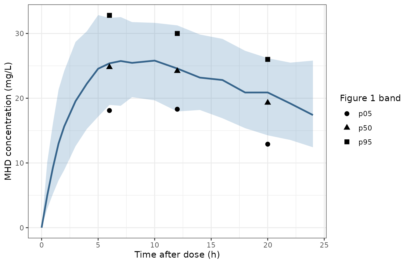

Replicates the right panel (Study 2) of Figure 1 of Jang 2021: simulated 5th, 50th and 95th percentiles after a single 30 mg/kg dose (shaded band and line), with the centres of the published simulated percentile bands as points. Residual error is included, as in the published VPC.


vpc_chk <- vpc |>
  filter(time %in% fig1$time) |>
  left_join(fig1, by = "time", suffix = c("", "_fig"))
# Cohort percentiles differ between rxode2 builds; the median must sit near
# the published band and the tails within a wider envelope.
stopifnot(
  all(abs(vpc_chk$p50 / vpc_chk$p50_fig - 1) < 0.15),
  all(abs(vpc_chk$p05 / vpc_chk$p05_fig - 1) < 0.30),
  all(abs(vpc_chk$p95 / vpc_chk$p95_fig - 1) < 0.30)
)

The Study 1 panel of Figure 1 is not replicated: it pools spot samples across the registry’s individual doses, regimens and last-dose times, which are not published.

PKNCA validation

Non-compartmental analysis on the model-predicted concentrations (no residual error): the single-dose profile over 0-24 h and one steady-state day (0-24 h, two doses) of twice-daily dosing.

nca_conc <- sim |>
  select(id, time, Cc = ipredSim, treatment) |>
  filter(!is.na(Cc))
nca_dose <- events |>
  filter(evid == 1L) |>
  select(id, time, amt, treatment)
nca_dose <- bind_rows(
  nca_dose,
  nca_dose |> filter(treatment == "Twice daily, steady state") |>
    mutate(time = 12)
)

conc_obj <- PKNCA::PKNCAconc(nca_conc, Cc ~ time | treatment + id,
                             concu = "mg/L", timeu = "h")
dose_obj <- PKNCA::PKNCAdose(nca_dose, amt ~ time | treatment + id,
                             doseu = "mg")
intervals <- data.frame(start = 0, end = 24, cmax = TRUE, tmax = TRUE,
                        cmin = TRUE, auclast = TRUE)
nca_res <- PKNCA::pk.nca(PKNCA::PKNCAdata(conc_obj, dose_obj,
                                          intervals = intervals))
summary(nca_res)
#>  Interval Start Interval End                 treatment   N AUClast (h*mg/L)
#>               0           24      30 mg/kg single dose 200       515 [9.19]
#>               0           24 Twice daily, steady state 200       559 [52.2]
#>  Cmax (mg/L) Cmin (mg/L)          Tmax (h)
#>  26.4 [7.58]          NC 8.00 [4.00, 20.0]
#>  24.7 [51.1] 21.0 [54.6] 16.0 [4.00, 17.0]
#> 
#> Caption: AUClast, Cmax, Cmin: geometric mean and geometric coefficient of variation; Tmax: median and range; N: number of subjects

Steady-state AUC over 24 h equals daily dose / (CL/F)

Jang 2021 computed each patient’s AUC as Dose / (CL/F) with the daily dose. For the steady-state cohort the NCA AUC over one 24 h day must reproduce that identity per subject, up to trapezoidal error on the 0.5 h grid.

ind_cl <- sim |>
  filter(treatment == "Twice daily, steady state") |>
  distinct(id, cl)
auc_chk <- as.data.frame(nca_res) |>
  filter(treatment == "Twice daily, steady state", PPTESTCD == "auclast") |>
  select(id, auc24 = PPORRES) |>
  left_join(ss_subj |> select(id, daily_dose), by = "id") |>
  left_join(ind_cl, by = "id") |>
  mutate(pct_diff = 100 * (auc24 / (daily_dose / cl) - 1))
stopifnot(
  nrow(auc_chk) == n_sub,
  abs(median(auc_chk$pct_diff)) < 1,
  quantile(abs(auc_chk$pct_diff), 0.9) < 2
)
summary(auc_chk$pct_diff)
#>      Min.   1st Qu.    Median      Mean   3rd Qu.      Max. 
#> -0.088344 -0.031451 -0.021383 -0.025394 -0.015728 -0.004436

Comparison with Jang 2021 Table 1

Table 1 reports, for the 447 registry patients, the mean individual MHD AUC (daily dose / (CL/F) from the post hoc CL/F) and the mean model-derived trough. Both are means, so the simulated steady-state cohort is summarised by its mean here rather than the median.

ss_nca <- as.data.frame(nca_res) |>
  filter(treatment == "Twice daily, steady state",
         PPTESTCD %in% c("auclast", "cmin")) |>
  group_by(PPTESTCD) |>
  summarise(PPORRES = mean(PPORRES), .groups = "drop")

published <- data.frame(auclast = 653.8, cmin = 12.75)
cmp <- nlmixr2lib::ncaComparisonTable(
  simulated = ss_nca,
  reference = published,
  units = c(auclast = "h*mg/L", cmin = "mg/L"),
  tolerance_pct = 20
)
knitr::kable(cmp, caption = paste(
  "Mean steady-state exposure over one 24 h day of twice-daily dosing:",
  "simulated cohort vs Jang 2021 Table 1 (447 registry patients).",
  "AUC0-last spans 0-24 h, i.e. the daily AUC."
))

Mean steady-state exposure over one 24 h day of twice-daily dosing: simulated cohort vs Jang 2021 Table 1 (447 registry patients). AUC0-last spans 0-24 h, i.e. the daily AUC.
NCA parameter	Reference	Simulated	% diff
Cmin (mg/L)	12.8	23.8	+86.5%*
AUClast (h*mg/L)	654	628	-4.0%


auc_sim <- ss_nca$PPORRES[ss_nca$PPTESTCD == "auclast"]
cmin_sim <- ss_nca$PPORRES[ss_nca$PPTESTCD == "cmin"]
stopifnot(abs(auc_sim / 653.8 - 1) < 0.15)
# The trough discrepancy described below is large, not cohort noise.
stopifnot(cmin_sim > 1.4 * 12.75)

# Typical 66 kg patient at steady state on 500 mg twice daily: ratio of the
# trough to the daily-average concentration.
typ_ss <- rxode2::rxSolve(
  mod_typ,
  bind_rows(
    tibble(id = 1L, time = 0, evid = 1L, amt = 500, ii = 12, ss = 1L,
           cmt = "depot"),
    tibble(id = 1L, time = 12, evid = 0L, amt = 0, ii = 0, ss = 0L,
           cmt = "central")
  ) |> mutate(WT = 66),
  returnType = "data.frame", maxsteps = 1e6
)
#> ℹ omega/sigma items treated as zero: 'etalcl', 'etalka'
trough_ratio <- typ_ss$Cc / (1000 / 24 / 1.65)
stopifnot(trough_ratio > 0.85, trough_ratio < 0.95)
round(c(mean_trough_sim = cmin_sim, typical_trough_to_average = trough_ratio), 2)
#>           mean_trough_sim typical_trough_to_average 
#>                     23.78                      0.91

The daily AUC agrees with Table 1. The trough does not: the simulated mean twice-daily trough is well above the 12.75 mg/L in Table 1. The two Table 1 columns are not consistent with each other under the published model either – with CL/F = 1.65 L/h and V/F = 59 L the half-life is about 25 h, so for the typical patient a twice-daily trough is about 90% of the daily-average concentration (AUC / 24 = 27 mg/L for the Table 1 mean AUC). Jang 2021 describes the trough only as “estimated using a simulation method”, without the regimen or timing used, so the discrepancy cannot be traced from the article. It is reported here and was not used to change any parameter. The mean observed spot MHD concentration in Table 1 (15.8 mg/L) is likewise below the daily-average concentration the model implies for the mean dose.

Adverse-event analysis (not extracted)

Jang 2021 related the individual MHD trough and AUC to dose-related adverse events with ROC cut-offs (dose-related adverse events: trough 12.27 mg/L, AUC 698.5 mg h/L; dizziness alone: trough 19.15 mg/L, AUC 940.5 mg h/L) and a multivariable logistic regression adjusted for age, sex and GFR (Table 3; for dizziness, OR 1.079 per mg/L of trough and 1.002 per mg h/L of AUC). The regression intercepts are not reported, so no probability model can be reconstructed; the cut-offs are thresholds, not a model. Neither is packaged.

Assumptions and deviations

Second IIV on ka, not V/F. Table 2 labels the 41.5 %CV “IIV V2/F”; the final-model control stream fixes the V variance to zero and estimates the ka variance. The control stream is followed, confirmed against the Figure 1 simulated bands above.
%CV to variance. Table 2 gives IIV as %CV of an exponential model; the variances use omega^2 = log(1 + CV^2). With omega^2 = CV^2 instead, the variances would be 0.0853 and 0.1722, a difference that does not affect any check above.
Negligible additive error omitted. The control stream’s error model is W = sqrt(THETA(6)^2 + THETA(7)^2 * IPRED^2) with THETA(6) fixed at 0.0001 ng/mL; the paper describes the error model as proportional, and the fixed additive term (1e-7 mg/L) is omitted.
Concentration units. The analysis dataset was in ng/mL (SC = V/1000 with doses in mg). The model reports mg/L; Table 2 prints the proportional error with a unit of ng/mL, which does not apply to a fractional SD.
Table 2 unit typo. The V/F typical value is printed with unit “L h-1”; it is a volume in L, as the equation line above it states.
Body weight of the Study 2 patients. Not reported; the virtual single-dose cohort uses the registry weight distribution.
Screened, not retained. Age, sex and enzyme-inducing co-medication (an estimated 7% increase in CL/F) were tested and not retained; they are listed in covariatesDataExcluded.
Trough and observed levels. See the comparison with Table 1 above: the published model reproduces the Table 1 AUC but not the Table 1 trough, and the article does not describe the trough simulation in enough detail to find the cause.