Avadomide-induced neutropenia QSP (Abbiati 2021)
Source:vignettes/articles/Abbiati_2021_avadomide.Rmd
Abbiati_2021_avadomide.RmdAvadomide (CC-122) is a cereblon E3-ligase modulator whose dose-limiting toxicity is neutropenia. Abbiati et al. (2021) built a quantitative systems pharmacology (QSP) model of the mechanism: avadomide degrades the transcription factor Ikaros, which produces a reversible, incomplete block of late neutrophil maturation in the bone marrow. The circulating count holds up while a marrow reservoir of mature neutrophils drains, and then falls. The model has three layers:
- a two-compartment oral PK model with a lag time;
- a sigmoid Emax PD model that scales the maturation rate between the second and third marrow transit stages (Eq. 9);
- a neutrophil life-cycle model (Eqs. 1-8): proliferating precursors -> transit 1 -> transit 2 -> transit 3 -> marrow reservoir -> circulation. The transit-2 -> transit-3 step has Michaelis-Menten form, and two power-law feedbacks act on it: proliferation responds to the transit-2 level, and marrow egress responds to the circulating count.
Every rate constant follows from homeostasis once the circulating-neutrophil half-life, the apoptosis rate and three disease-specific parameters are chosen. The authors refitted those three parameters (gamma, the reservoir-to-circulation ratio and the KM fraction) to each disease cohort. Each Table I column is therefore packaged as its own model:
mod_gbm <- rxode2::rxode(readModelDb("Abbiati_2021_avadomide_gbm"))
mod_dlbcl <- rxode2::rxode(readModelDb("Abbiati_2021_avadomide_dlbcl"))
mod_mm <- rxode2::rxode(readModelDb("Abbiati_2021_avadomide_mm"))
Model and source
- Citation: Abbiati RA, Pourdehnad M, Carrancio S, Pierce DW, Kasibhatla S, McConnell M, Trotter MWB, Loos R, Santini CC, Ratushny AV. Quantitative Systems Pharmacology Modeling of Avadomide-Induced Neutropenia Enables Virtual Clinical Dose and Schedule Finding Studies. AAPS J. 2021;23(5):103. doi:10.1208/s12248-021-00623-8. Correction: AAPS J. 2022;24(1):29. doi:10.1208/s12248-021-00673-y (replaces the supplementary material; no value in the main text changed).
- Description (DLBCL file): QSP. Avadomide (CC-122)-induced neutropenia in adults with diffuse large B-cell lymphoma (DLBCL); median DLBCL-cohort parameter set. A two-compartment oral PK model with first-order absorption and a lag time drives a sigmoid Emax partial block of neutrophil maturation (cereblon-mediated Ikaros degradation), which acts on a Michaelis-Menten transfer from the second to the third bone-marrow maturation stage of a neutrophil life-cycle model: proliferating precursors -> three transit stages -> bone-marrow reservoir of mature neutrophils -> circulating neutrophils (ANC). Two power-law feedbacks regulate proliferation (on transit-2 level) and marrow egress (on ANC). Every rate constant is back-calculated from homeostasis. Deterministic mechanism model: the authors built virtual patients by resampling the empirical distributions of baseline ANC, gamma, the reservoir-to-circulation ratio and the KM fraction rather than by estimating IIV or residual error, so no etas and no error model are encoded. Sibling files carry the glioblastoma (Abbiati_2021_avadomide_gbm) and multiple myeloma (Abbiati_2021_avadomide_mm) parameter sets of the same structure.
- Article: https://doi.org/10.1208/s12248-021-00623-8 (open access in PMC, PMC8397660)
- Correction: https://doi.org/10.1208/s12248-021-00673-y. The notice states only that the article “has been updated to add the correct supplementary material”. The supplement used here is the corrected deposit: its Table S.III reproduces the main-text Table II row for row.
Population
The ANC data come from the first-in-human trial NCT01421524 (CC-122-ST-001), restricted to the first 28-day treatment cycle. ANC measured after the first G-CSF administration were removed. Individual profiles were resampled into 4-day windows before fitting (Supplementary Materials, “Figure 3 data processing details”).
- Glioblastoma (GBM), n = 37 (Figure 2: 3 mg QD n = 22, 4 mg QD n = 4, 5 mg QD n = 3, 5 mg 5/7 n = 5, 6 mg 5/7 n = 3). These patients had no prior marrow-depleting therapy, so they were fitted first. That fit estimated the PD parameters EC50 and n, and those values were then held for every other cohort.
- Diffuse large B-cell lymphoma (DLBCL), n = 54 (4 mg 5/7 n = 30 + 4, 3 mg 5/7 n = 12, 5 mg 5/7 n = 5, 4 mg 21/28 n = 3). The authors refitted the median profile, then refitted each patient individually to build the virtual population (Figure 4). Two further DLBCL cohorts (3 mg QD n = 18; 3 mg 5/7 n = 14) were reserved for validation (Figure 5).
- Multiple myeloma (MM), n = 37, some with dexamethasone. The paper reports the MM column of Table I but shows no MM fit or MM simulation.
No age, sex or body-weight summary is reported. The same information
is available programmatically,
e.g. mod_dlbcl$population.
Source trace
Every ini() value carries an in-file comment naming its
source. The table collects them. Table I rows marked type “C” (computed)
are derived inside model() from the homeostasis equations.
They are not free parameters.
| Parameter / equation | GBM | DLBCL | MM | Source |
|---|---|---|---|---|
lka (k_abs, 1/h) |
5.5 | 5.5 | 5.5 | Supplement, “Avadomide PK” table |
ltlag (Abs_lag, h) |
0.406 | 0.406 | 0.406 | Supplement, “Avadomide PK” table |
lkel (k_el, 1/h) |
0.0708 | 0.0708 | 0.0708 | Supplement, “Avadomide PK” table |
lk12 (1/h) |
0.0265 | 0.0265 | 0.0265 | Supplement, “Avadomide PK” table |
lk21 (1/h) |
0.0195 | 0.0195 | 0.0195 | Supplement, “Avadomide PK” table |
lvc (V/F, L) |
48.7 | 48.7 | 48.7 | Back-solved from the deposited PK profile (Supplementary file MOESM2); see Assumptions |
lec50 (EC50,PD, ng/mL) |
15 (estimated) | 15 (held) | 15 (held) | Table I |
lhill (n_PD) |
2 (estimated) | 2 (held) | 2 (held) | Table I |
emax (Emax,PD) |
0.9 | 0.9 | 0.9 | Table I (type A) |
lgamma |
0.02 | 0.01 | 0.017 | Table I (type R) |
lbeta |
20 | 20 | 20 | Table I (type A) |
lcirc0 (Circ0, 10^9 cells/L) |
4.5 | 4.5 | 4.5 | Table I (example typical value; patient-specific input) |
lthalf_circ (t1/2, h) |
30 | 30 | 30 | Table I; Results, “Model Parameterization” |
lkd_mat (kd, 1/h) |
0.001 | 0.001 | 0.001 | Table I (type A) |
lratio_reserv (Reserv0/Circ0) |
3 | 2.5 | 2.5 | Table I (type R) |
lkm_frac (KM,fraction) |
0.6 | 0.1 | 0.45 | Table I (type R) |
kelim = log(2)/t1/2; kout,
ktr4, ktr3, ktr2,
ktr1, kprol, KM,
Vmax
|
derived | derived | derived | Table I type-C formulas; supplementary R script (MOESM3) |
d/dt(prol) … d/dt(circ)
|
Eqs. 1-6; supplementary R script | |||
Feedback proliferation (Tran0/transit2)^gamma
|
Eq. 7 | |||
Feedback egress (Circ0/circ)^beta
|
Eq. 8 | |||
eff_mat = 1 - Emax C^n / (EC50^n + C^n) |
Eq. 9 | |||
| Initial conditions (all stages = Circ0, reservoir = ratio x Circ0) | Results, “Model Parameterization”; R script |
The model equations match the authors’ supplementary deSolve script line by line.
Homeostasis without drug
Every rate constant is back-calculated so that all six marrow and blood stages sit exactly at their initial values without drug. A drug-free solve must hold them there.
ss_check <- function(mod) {
  s <- rxode2::rxSolve(mod, events = rxode2::et(seq(0, 28 * 24, by = 24)))
  s <- as.data.frame(s)
  st <- c("prol", "transit1", "transit2", "transit3", "reservoir", "circ")
  max(abs(sweep(as.matrix(s[, st]), 2, unlist(s[1, st]), "/") - 1))
}
ss_dev <- c(
  GBM = ss_check(mod_gbm),
  DLBCL = ss_check(mod_dlbcl),
  MM = ss_check(mod_mm)
)
ss_dev
#>   GBM DLBCL    MM
#>     0     0     0
# The drift is pure numerical error of the solver, so a tight bound applies.
stopifnot(all(ss_dev < 1e-6))
Avadomide PK: exposure over the first cycle
The PK model has no between-subject variability, so one typical subject per regimen gives the exposure the authors report. Table II and Table S.III list AUC and Cmax over the first 28-day cycle. Doses run from day 0, and the schedule “a/b” means a dosing days in every b-day block. The AUC column of Table II is labelled “ng/ml*h”, but its values are in ng/mL x day (see Assumptions). The published values are therefore multiplied by 24 before the comparison.
# Dosing days for an "on/period" schedule within the analysis window.
schedule_days <- function(on, period, n_days) {
  d <- seq(0, n_days - 1)
  d[(d %% period) < on]
}

pk_regimens <- tibble::tribble(
  ~schedule, ~on, ~period, ~dose,
  "3/7", 3, 7, 4,
  "5/7", 5, 7, 4,
  "7/14", 7, 14, 4,
  "14/28", 14, 28, 4,
  "21/28", 21, 28, 4,
  "28/28", 28, 28, 4,
  "5/7", 5, 7, 2,
  "5/7", 5, 7, 6,
  "5/7", 5, 7, 8
) |>
  mutate(treatment = paste(dose, "mg", schedule))

# A dense grid resolves the sharp absorption peak (ka = 5.5 1/h after a
# 0.4 h lag); a coarse grid understates both Cmax and AUC.
pk_times <- sort(unique(c(seq(0, 28 * 24, by = 0.05))))

pk_sim <- lapply(seq_len(nrow(pk_regimens)), function(i) {
  r <- pk_regimens[i, ]
  ev <- rxode2::et(
    amt = r$dose,
    time = schedule_days(r$on, r$period, 28) * 24,
    cmt = "depot"
  ) |>
    rxode2::et(pk_times)
  s <- as.data.frame(rxode2::rxSolve(mod_dlbcl, events = ev))
  tibble(id = i, treatment = r$treatment, time = s$time, Cc = s$Cc)
}) |>
  bind_rows()

pk_doses <- lapply(seq_len(nrow(pk_regimens)), function(i) {
  r <- pk_regimens[i, ]
  tibble(
    id = i,
    treatment = r$treatment,
    time = schedule_days(r$on, r$period, 28) * 24,
    amt = r$dose
  )
}) |>
  bind_rows()
conc_obj <- PKNCA::PKNCAconc(
  pk_sim |> dplyr::filter(!is.na(Cc)),
  Cc ~ time | treatment + id
)
dose_obj <- PKNCA::PKNCAdose(pk_doses, amt ~ time | treatment + id)
intervals <- data.frame(
  start = 0,
  end = 28 * 24,
  cmax = TRUE,
  auclast = TRUE
)
nca_res <- PKNCA::pk.nca(PKNCA::PKNCAdata(conc_obj, dose_obj, intervals = intervals))

# Table II (A: 4 mg, all schedules; B: 5/7 at 2, 6, 8 mg); AUC printed in
# ng/mL x day, converted to ng*h/mL here.
published_pk <- tibble::tribble(
  ~treatment, ~auc_day, ~cmax,
  "4 mg 3/7", 571, 91,
  "4 mg 5/7", 945, 96,
  "4 mg 7/14", 672, 96,
  "4 mg 14/28", 676, 98,
  "4 mg 21/28", 1010, 98,
  "4 mg 28/28", 1303, 98,
  "2 mg 5/7", 472, 48,
  "6 mg 5/7", 1417, 143,
  "8 mg 5/7", 1889, 191
) |>
  mutate(auclast = auc_day * 24) |>
  select(treatment, cmax, auclast)

pk_cmp <- nlmixr2lib::ncaComparisonTable(
  simulated = nca_res,
  reference = published_pk,
  by = "treatment",
  units = c(cmax = "ng/mL", auclast = "ng*h/mL"),
  tolerance_pct = 20
)
knitr::kable(
  pk_cmp,
  caption = paste(
    "Simulated first-cycle exposure vs. Table II. * differs from the",
    "published value by >20%."
  )
)| NCA parameter | treatment | Reference | Simulated | % diff |
|---|---|---|---|---|
| Cmax (ng/mL) | 4 mg 3/7 | 91 | 91.4 | +0.4% |
| Cmax (ng/mL) | 4 mg 5/7 | 96 | 95.5 | -0.5% |
| Cmax (ng/mL) | 4 mg 7/14 | 96 | 95.8 | -0.2% |
| Cmax (ng/mL) | 4 mg 14/28 | 98 | 97.5 | -0.5% |
| Cmax (ng/mL) | 4 mg 21/28 | 98 | 97.7 | -0.3% |
| Cmax (ng/mL) | 4 mg 28/28 | 98 | 97.7 | -0.3% |
| Cmax (ng/mL) | 2 mg 5/7 | 48 | 47.8 | -0.5% |
| Cmax (ng/mL) | 6 mg 5/7 | 143 | 143 | +0.2% |
| Cmax (ng/mL) | 8 mg 5/7 | 191 | 191 | +0.0% |
| AUClast (ng*h/mL) | 4 mg 3/7 | 13700 | 13700 | +0.0% |
| AUClast (ng*h/mL) | 4 mg 5/7 | 22700 | 22700 | -0.0% |
| AUClast (ng*h/mL) | 4 mg 7/14 | 16100 | 16100 | +0.0% |
| AUClast (ng*h/mL) | 4 mg 14/28 | 16200 | 16200 | +0.0% |
| AUClast (ng*h/mL) | 4 mg 21/28 | 24200 | 24200 | +0.0% |
| AUClast (ng*h/mL) | 4 mg 28/28 | 31300 | 31300 | +0.1% |
| AUClast (ng*h/mL) | 2 mg 5/7 | 11300 | 11300 | +0.1% |
| AUClast (ng*h/mL) | 6 mg 5/7 | 34000 | 34000 | +0.0% |
| AUClast (ng*h/mL) | 8 mg 5/7 | 45300 | 45300 | +0.0% |
pk_sim_wide <- as.data.frame(nca_res$result) |>
  dplyr::filter(PPTESTCD %in% c("cmax", "auclast")) |>
  select(treatment, PPTESTCD, PPORRES) |>
  tidyr::pivot_wider(names_from = PPTESTCD, values_from = PPORRES) |>
  inner_join(published_pk, by = "treatment", suffix = c("_sim", "_pub"))
stopifnot(nrow(pk_sim_wide) == nrow(published_pk))
pk_pct <- with(pk_sim_wide, c(
  100 * (auclast_sim / auclast_pub - 1),
  100 * (cmax_sim / cmax_pub - 1)
))
round(range(pk_pct), 2)
#> [1] -0.52  0.42
# Deterministic: no random effects in the PK. Published values are rounded
# to integers (Cmax 48 carries up to 1% rounding) and the 28/28 AUC differs
# between Table II (1303) and Table S.III (1304). Observed: -0.52% to +0.42%.
stopifnot(all(abs(pk_pct) < 1.5))
The back-solved V/F reproduces every first-cycle AUC and Cmax in Table II to within rounding. Only V/F was calibrated, and only against the 5 mg 5/7 profile the authors deposited. The dose and schedule scaling across the other rows is an out-of-sample check of the PK constants and of the schedule reading.
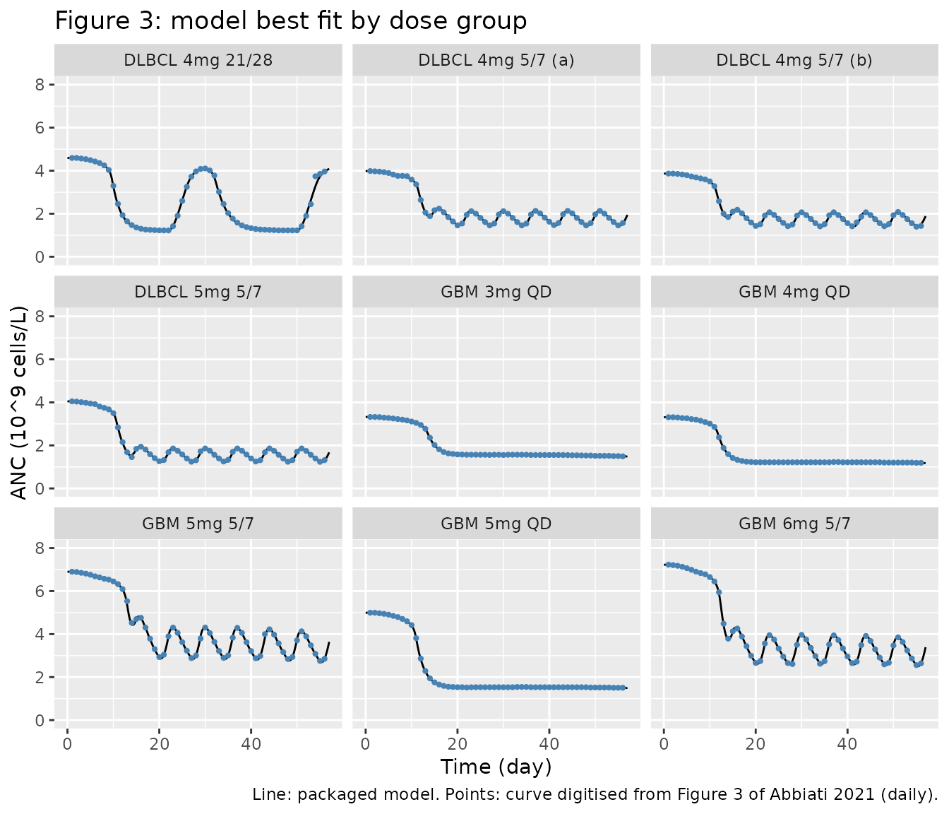
Figure 3: typical-patient fits by cohort
Figure 3 overlays the model best fit (black line) on the ANC of each
GBM and DLBCL dose group. The figure is vector graphics, so the
maintainers extracted the plotted curves exactly from the PDF and
resampled them at daily points, day 1 to 56. Dosing starts on day 1, and
each curve’s starting value is the panel’s baseline ANC, used here as
lcirc0. The authors’ R script uses the same convention: it
reproduces the GBM 5 mg 5/7 panel with Circ0 = 7e9 and the DLBCL 5 mg
5/7 panel with 4e9. (The x-axis of Figure 3 reads “time [h]”, but the
scale is days.)
# Digitised Figure 3 best-fit curves: ANC (10^9 cells/L) at days 1, 2, ..., 56.
fig3_digitised <- list(
  "GBM 3mg QD" = c(3.323, 3.323, 3.314, 3.291, 3.275, 3.250, 3.223, 3.198, 3.160, 3.110, 3.047, 2.952, 2.772, 2.355, 2.018, 1.819, 1.692, 1.629, 1.604, 1.579, 1.574, 1.566, 1.566, 1.566, 1.563, 1.565, 1.555, 1.566, 1.564, 1.554, 1.566, 1.566, 1.566, 1.566, 1.566, 1.554, 1.554, 1.554, 1.554, 1.554, 1.554, 1.554, 1.554, 1.548, 1.541, 1.541, 1.535, 1.529, 1.529, 1.516, 1.516, 1.516, 1.516, 1.505, 1.504, 1.491),
  "GBM 4mg QD" = c(3.310, 3.310, 3.298, 3.272, 3.260, 3.223, 3.199, 3.147, 3.084, 3.009, 2.859, 2.376, 1.885, 1.592, 1.416, 1.328, 1.278, 1.240, 1.227, 1.215, 1.215, 1.215, 1.215, 1.215, 1.215, 1.215, 1.215, 1.215, 1.215, 1.215, 1.215, 1.215, 1.215, 1.215, 1.215, 1.215, 1.227, 1.227, 1.215, 1.215, 1.215, 1.215, 1.215, 1.215, 1.215, 1.215, 1.215, 1.202, 1.202, 1.202, 1.202, 1.202, 1.202, 1.202, 1.190, 1.190),
  "GBM 5mg QD" = c(4.992, 4.992, 4.966, 4.941, 4.904, 4.846, 4.791, 4.703, 4.594, 4.415, 3.809, 2.861, 2.284, 1.940, 1.754, 1.654, 1.591, 1.554, 1.541, 1.529, 1.529, 1.516, 1.527, 1.529, 1.529, 1.529, 1.529, 1.529, 1.529, 1.529, 1.529, 1.529, 1.541, 1.541, 1.541, 1.529, 1.529, 1.529, 1.529, 1.529, 1.529, 1.529, 1.529, 1.529, 1.529, 1.529, 1.529, 1.529, 1.516, 1.516, 1.516, 1.516, 1.514, 1.504, 1.504, 1.504),
  "GBM 6mg 5/7" = c(7.225, 7.205, 7.175, 7.130, 7.064, 6.989, 6.904, 6.836, 6.777, 6.648, 6.447, 5.945, 4.483, 3.785, 4.127, 4.257, 3.888, 3.439, 2.993, 2.658, 2.744, 3.563, 3.948, 3.745, 3.329, 2.953, 2.651, 2.606, 3.500, 3.963, 3.746, 3.359, 2.976, 2.621, 2.738, 3.519, 3.938, 3.720, 3.331, 2.960, 2.650, 2.715, 3.490, 3.913, 3.681, 3.292, 2.907, 2.593, 2.671, 3.469, 3.847, 3.629, 3.239, 2.867, 2.557, 2.639),
  "GBM 5mg 5/7" = c(6.899, 6.886, 6.849, 6.811, 6.758, 6.686, 6.633, 6.573, 6.529, 6.447, 6.322, 6.091, 5.532, 4.522, 4.697, 4.756, 4.301, 3.782, 3.302, 2.933, 3.042, 3.899, 4.301, 4.057, 3.624, 3.228, 2.882, 3.004, 3.796, 4.302, 4.047, 3.637, 3.215, 2.894, 3.009, 3.831, 4.289, 4.054, 3.619, 3.211, 2.877, 2.980, 3.998, 4.221, 3.973, 3.567, 3.160, 2.840, 2.934, 3.709, 4.129, 3.896, 3.479, 3.083, 2.752, 2.849),
  "DLBCL 4mg 5/7 (a)" = c(3.984, 3.971, 3.958, 3.932, 3.893, 3.821, 3.757, 3.759, 3.745, 3.587, 3.365, 2.641, 2.059, 1.885, 2.160, 2.235, 2.067, 1.842, 1.639, 1.458, 1.545, 1.946, 2.118, 2.002, 1.807, 1.612, 1.457, 1.543, 1.963, 2.118, 2.002, 1.807, 1.613, 1.458, 1.542, 1.963, 2.131, 2.015, 1.820, 1.627, 1.471, 1.570, 1.976, 2.131, 2.015, 1.807, 1.613, 1.457, 1.563, 1.969, 2.131, 2.002, 1.807, 1.615, 1.457, 1.567),
  "DLBCL 5mg 5/7" = c(4.049, 4.036, 4.010, 3.984, 3.945, 3.918, 3.806, 3.747, 3.673, 3.498, 2.836, 2.151, 1.681, 1.455, 1.840, 1.937, 1.807, 1.587, 1.406, 1.263, 1.320, 1.678, 1.859, 1.750, 1.578, 1.392, 1.241, 1.310, 1.726, 1.859, 1.755, 1.561, 1.393, 1.251, 1.330, 1.698, 1.859, 1.752, 1.574, 1.393, 1.251, 1.313, 1.678, 1.859, 1.747, 1.561, 1.388, 1.240, 1.316, 1.704, 1.859, 1.743, 1.561, 1.393, 1.237, 1.316),
  "DLBCL 4mg 21/28" = c(4.593, 4.593, 4.565, 4.537, 4.489, 4.429, 4.354, 4.246, 4.034, 3.298, 2.459, 1.935, 1.644, 1.471, 1.364, 1.302, 1.263, 1.251, 1.237, 1.225, 1.225, 1.223, 1.420, 1.907, 2.595, 3.250, 3.724, 3.968, 4.082, 4.103, 4.012, 3.777, 3.020, 2.456, 2.032, 1.773, 1.587, 1.456, 1.378, 1.328, 1.289, 1.268, 1.257, 1.246, 1.237, 1.225, 1.225, 1.225, 1.225, 1.225, 1.418, 1.902, 2.442, 3.740, 3.852, 3.962),
  "DLBCL 4mg 5/7 (b)" = c(3.867, 3.867, 3.850, 3.824, 3.790, 3.733, 3.686, 3.642, 3.595, 3.504, 3.283, 2.581, 2.000, 1.844, 2.092, 2.183, 2.017, 1.792, 1.593, 1.431, 1.512, 1.914, 2.067, 1.946, 1.755, 1.574, 1.419, 1.500, 1.911, 2.067, 1.937, 1.755, 1.561, 1.411, 1.514, 1.924, 2.067, 1.937, 1.750, 1.561, 1.416, 1.598, 1.862, 2.067, 1.937, 1.746, 1.561, 1.417, 1.520, 1.928, 2.080, 1.940, 1.749, 1.557, 1.396, 1.433)
)
fig3_panels <- tibble::tribble(
  ~panel, ~cohort, ~dose, ~on, ~period,
  "GBM 3mg QD", "GBM", 3, 1, 1,
  "GBM 4mg QD", "GBM", 4, 1, 1,
  "GBM 5mg QD", "GBM", 5, 1, 1,
  "GBM 6mg 5/7", "GBM", 6, 5, 7,
  "GBM 5mg 5/7", "GBM", 5, 5, 7,
  "DLBCL 4mg 5/7 (a)", "DLBCL", 4, 5, 7,
  "DLBCL 5mg 5/7", "DLBCL", 5, 5, 7,
  "DLBCL 4mg 21/28", "DLBCL", 4, 21, 28,
  "DLBCL 4mg 5/7 (b)", "DLBCL", 4, 5, 7
)
stopifnot(setequal(fig3_panels$panel, names(fig3_digitised)))
fig3_sim <- lapply(seq_len(nrow(fig3_panels)), function(i) {
  p <- fig3_panels[i, ]
  mod <- if (p$cohort == "GBM") mod_gbm else mod_dlbcl
  dig <- fig3_digitised[[p$panel]]
  ev <- rxode2::et(
    amt = p$dose,
    time = 24 * (1 + schedule_days(p$on, p$period, 56)),
    cmt = "depot"
  ) |>
    rxode2::et(seq(0, 57 * 24, by = 2))
  s <- as.data.frame(rxode2::rxSolve(
    mod,
    events = ev, params = c(lcirc0 = log(dig[1])),
    method = "cvode", atol = 1e-10, rtol = 1e-10
  ))
  tibble(panel = p$panel, day = s$time / 24, ANC = s$ANC)
}) |>
  bind_rows()

fig3_dig <- lapply(names(fig3_digitised), function(nm) {
  tibble(panel = nm, day = seq_along(fig3_digitised[[nm]]), ANC_pub = fig3_digitised[[nm]])
}) |>
  bind_rows()

fig3_cmp <- fig3_dig |>
  group_by(panel) |>
  mutate(ANC_sim = approx(
    fig3_sim$day[fig3_sim$panel == panel[1]],
    fig3_sim$ANC[fig3_sim$panel == panel[1]],
    day
  )$y) |>
  ungroup() |>
  mutate(pct_diff = 100 * (ANC_sim / ANC_pub - 1))

fig3_summary <- fig3_cmp |>
  group_by(panel) |>
  summarise(
    median_abs_pct = median(abs(pct_diff)),
    p90_abs_pct = unname(quantile(abs(pct_diff), 0.9)),
    nadir_pub = min(ANC_pub),
    nadir_sim = min(ANC_sim),
    .groups = "drop"
  )
fig3_summary |>
  dplyr::rename(
    "Figure 3 panel" = panel,
    "Median |% diff|" = median_abs_pct,
    "90th pct |% diff|" = p90_abs_pct,
    "Published nadir (10^9/L)" = nadir_pub,
    "Simulated nadir (10^9/L)" = nadir_sim
  ) |>
knitr::kable(digits = 2, caption = "Packaged model vs. digitised Figure 3 best-fit curves.")| Figure 3 panel | Median |% diff| | 90th pct |% diff| | Published nadir (10^9/L) | Simulated nadir (10^9/L) |
|---|---|---|---|---|
| DLBCL 4mg 21/28 | 0.33 | 2.42 | 1.22 | 1.22 |
| DLBCL 4mg 5/7 (a) | 0.34 | 1.02 | 1.46 | 1.46 |
| DLBCL 4mg 5/7 (b) | 0.45 | 1.45 | 1.40 | 1.42 |
| DLBCL 5mg 5/7 | 0.31 | 1.23 | 1.24 | 1.25 |
| GBM 3mg QD | 0.20 | 0.57 | 1.49 | 1.50 |
| GBM 4mg QD | 0.32 | 0.92 | 1.19 | 1.18 |
| GBM 5mg 5/7 | 0.34 | 1.14 | 2.75 | 2.73 |
| GBM 5mg QD | 0.27 | 0.74 | 1.50 | 1.50 |
| GBM 6mg 5/7 | 0.22 | 0.88 | 2.56 | 2.55 |
ggplot() +
  geom_line(data = fig3_sim, aes(day, ANC), colour = "black") +
  geom_point(data = fig3_dig, aes(day, ANC_pub), colour = "steelblue", size = 0.8) +
  facet_wrap(~panel, ncol = 3) +
  coord_cartesian(xlim = c(0, 57), ylim = c(0, 8)) +
  labs(
    x = "Time (day)", y = "ANC (10^9 cells/L)",
    title = "Figure 3: model best fit by dose group",
    caption = paste(
      "Line: packaged model. Points: curve digitised from Figure 3 of",
      "Abbiati 2021 (daily)."
    )
  )
# Deterministic comparison (no random effects), limited only by the
# digitisation of a vector figure and by where daily points fall on the
# weekly 5/7 oscillation. Observed: median 0.20-0.45% per panel, 90th
# percentile 0.57-2.42%.
stopifnot(
  nrow(fig3_cmp) == 9 * 56,
  !anyNA(fig3_cmp$ANC_sim),
  all(fig3_summary$median_abs_pct < 1),
  all(fig3_summary$p90_abs_pct < 4)
)
The packaged GBM and DLBCL parameter sets reproduce all nine best-fit curves. The one visible difference is in the second “DLBCL 4mg 5/7” panel. Its weekend troughs, read at the full resolution of the vector figure, dip to 1.27 x 10^9/L against 1.40 in the simulation, while the daily points above agree. That panel repeats a dose group already shown in panel (a), so its fit probably used a slightly different input (see Assumptions).
Virtual DLBCL cohort (Figure 4) and dose / schedule exploration (Table II)
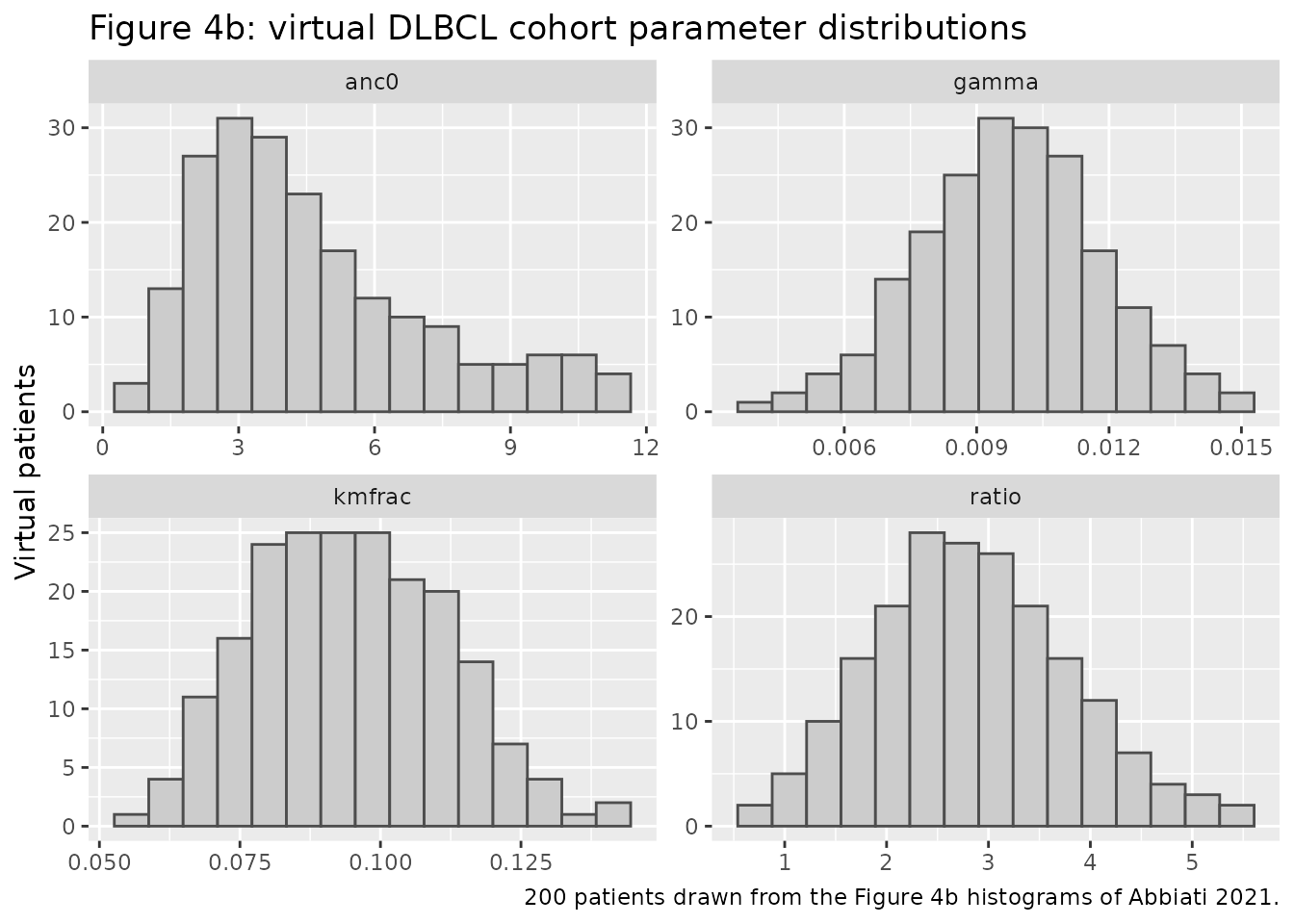
The authors built virtual DLBCL patients by drawing four parameters independently from kernel-density estimates of the individual fits: baseline ANC, gamma, the reservoir ratio and the KM fraction. Figure 4b shows the resulting 1000-patient histograms. The maintainers extracted the bar heights exactly from the vector figure. Each panel sums to 1000 patients, which checks the extraction. The cohort below draws 200 patients from those histograms by stratified (Latin-hypercube) sampling, uniform within each bar. The other parameters keep their DLBCL values from Table I. The same 200 patients receive every regimen, as in the paper.
# Figure 4b histograms (bin breaks; counts of the 1000 virtual patients).
# ANC baseline in 10^9 cells/L.
fig4b_bins <- list(
  gamma = list(
    breaks = c(0.0034989, 0.004275, 0.0050381, 0.0058142, 0.0065772, 0.0073534, 0.008117, 0.0088926, 0.0096562, 0.010432, 0.011195, 0.011971, 0.012735, 0.013511, 0.014274, 0.01505),
    count = c(4, 7, 18, 28, 58, 92, 115, 153, 150, 143, 97, 56, 42, 24, 13)
  ),
  ratio = list(
    breaks = c(0.59752, 0.93049, 1.2579, 1.5908, 1.9182, 2.2511, 2.5787, 2.9115, 3.2391, 3.5718, 3.8994, 4.2324, 4.5597, 4.8927, 5.2203, 5.553),
    count = c(13, 25, 54, 79, 102, 140, 136, 122, 103, 86, 58, 33, 24, 15, 10)
  ),
  kmfrac = list(
    breaks = c(0.055009, 0.060957, 0.066806, 0.072754, 0.078607, 0.084455, 0.090404, 0.096352, 0.1022, 0.10805, 0.114, 0.11995, 0.1258, 0.13174, 0.1376, 0.14345),
    count = c(10, 25, 67, 80, 122, 123, 121, 117, 98, 101, 67, 32, 17, 10, 10)
  ),
  anc0 = list(
    breaks = c(0.60784, 1.3332, 2.0464, 2.7601, 3.4854, 4.1986, 4.924, 5.6489, 6.3625, 7.0762, 7.8011, 8.5265, 9.2396, 9.9533, 10.679, 11.392),
    count = c(28, 85, 144, 151, 132, 103, 75, 57, 51, 39, 28, 25, 26, 26, 30)
  )
)
stopifnot(all(vapply(fig4b_bins, function(b) sum(b$count), numeric(1)) == 1000))
# Inverse CDF of a histogram, linear within each bar.
histogram_quantile <- function(u, breaks, count) {
  cdf <- c(0, cumsum(count)) / sum(count)
  stats::approx(cdf, breaks, xout = u, ties = "ordered")$y
}
latin_hypercube <- function(n) (sample.int(n) - stats::runif(n)) / n

set.seed(20210827)
n_vp <- 200
vp <- tibble(
  gamma = histogram_quantile(latin_hypercube(n_vp), fig4b_bins$gamma$breaks, fig4b_bins$gamma$count),
  ratio = histogram_quantile(latin_hypercube(n_vp), fig4b_bins$ratio$breaks, fig4b_bins$ratio$count),
  kmfrac = histogram_quantile(latin_hypercube(n_vp), fig4b_bins$kmfrac$breaks, fig4b_bins$kmfrac$count),
  anc0 = histogram_quantile(latin_hypercube(n_vp), fig4b_bins$anc0$breaks, fig4b_bins$anc0$count)
)
# Per-patient overrides of the typical values (the thetas are log-scale).
vp_params <- data.frame(
  lgamma = log(vp$gamma),
  lratio_reserv = log(vp$ratio),
  lkm_frac = log(vp$kmfrac),
  lcirc0 = log(vp$anc0)
)
summary(vp)
#>      gamma              ratio            kmfrac             anc0
#>  Min.   :0.003976   Min.   :0.7082   Min.   :0.05571   Min.   : 0.6351
#>  1st Qu.:0.008403   1st Qu.:2.1781   1st Qu.:0.08189   1st Qu.: 2.7280
#>  Median :0.009775   Median :2.7870   Median :0.09401   Median : 3.9790
#>  Mean   :0.009773   Mean   :2.8472   Mean   :0.09475   Mean   : 4.6340
#>  3rd Qu.:0.011088   3rd Qu.:3.4896   3rd Qu.:0.10726   3rd Qu.: 6.0386
#>  Max.   :0.014898   Max.   :5.4384   Max.   :0.14145   Max.   :11.2733
vp |>
  tidyr::pivot_longer(everything(), names_to = "parameter", values_to = "value") |>
  ggplot(aes(value)) +
  geom_histogram(bins = 15, fill = "grey80", colour = "grey30") +
  facet_wrap(~parameter, scales = "free") +
  labs(
    x = NULL, y = "Virtual patients",
    title = "Figure 4b: virtual DLBCL cohort parameter distributions",
    caption = "200 patients drawn from the Figure 4b histograms of Abbiati 2021."
  )
The endpoints follow the Methods and the note on Table S.III.
- Grade 3 / grade 4 neutropenia: ANC below 1.0 / 0.5 x 10^9/L, with onset in the first 28 days.
- 7-day events: the ANC stays below the threshold for at least 7 consecutive days. Onset must fall in the first 28 days, and the profile is followed to day 35.
- Recovery: at least one ANC at or above the grade-2 upper threshold (1.5 x 10^9/L) after the first toxicity onset, within the first cycle. Table II reports it as a percentage of all virtual patients; for example, 12.5% of the 19% with grade 3 on 4 mg 7/14.
- Time to recover: mean days from the first onset to that first ANC.
neutropenia_endpoints <- function(t_day, anc, threshold) {
  below <- anc < threshold
  onset_idx <- which(below & t_day <= 28)
  if (length(onset_idx) == 0) {
    return(c(any = 0, d7 = 0, recovered = 0, t_recover = NA_real_))
  }
  runs <- rle(below)
  run_end <- cumsum(runs$lengths)
  run_start <- run_end - runs$lengths + 1
  keep <- runs$values & t_day[run_start] <= 28
  # Duration = time to the first sample back above the threshold (or the end
  # of the day-35 window).
  run_dur <- t_day[pmin(run_end[keep] + 1, length(t_day))] - t_day[run_start[keep]]
  t_onset <- t_day[onset_idx[1]]
  rec_idx <- which(t_day > t_onset & t_day <= 28 & anc >= 1.5)
  c(
    any = 1,
    d7 = as.numeric(any(run_dur >= 7)),
    recovered = as.numeric(length(rec_idx) > 0),
    t_recover = if (length(rec_idx) > 0) t_day[rec_idx[1]] - t_onset else NA_real_
  )
}

table2_regimens <- tibble::tribble(
  ~panel, ~schedule, ~on, ~period, ~dose,
  "A", "3/7", 3, 7, 4,
  "A", "5/7", 5, 7, 4,
  "A", "7/14", 7, 14, 4,
  "A", "14/28", 14, 28, 4,
  "A", "21/28", 21, 28, 4,
  "A", "28/28", 28, 28, 4,
  "B", "5/7", 5, 7, 2,
  "B", "5/7", 5, 7, 3,
  "B", "5/7", 5, 7, 5,
  "B", "5/7", 5, 7, 6,
  "B", "5/7", 5, 7, 7,
  "B", "5/7", 5, 7, 8
) |>
  mutate(treatment = paste(dose, "mg", schedule))

vp_sim <- lapply(seq_len(nrow(table2_regimens)), function(i) {
  r <- table2_regimens[i, ]
  # Dosing continues past day 28 (the next cycle) so the day-35 window used
  # for the 7-day endpoints sees the real schedule.
  ev <- rxode2::et(
    amt = r$dose,
    time = schedule_days(r$on, r$period, 36) * 24,
    cmt = "depot"
  ) |>
    rxode2::et(seq(0, 36 * 24, by = 2))
  # The egress feedback exponent (beta = 20) makes the system extremely stiff
  # once the ANC falls well below baseline: the egress factor (Circ0/circ)^20
  # reaches ~1e14 and the reservoir is emptied to ~1e-14. The default
  # liblsoda solver fails for part of the cohort on the long-holiday and
  # high-dose schedules (from 2% to half of the patients, depending on the
  # tolerance); the SUNDIALS CVODE BDF solver solves them all, and agrees with
  # liblsoda to ~1e-7 where both succeed.
  s <- as.data.frame(rxode2::rxSolve(
    mod_dlbcl,
    params = vp_params, events = ev,
    method = "cvode", atol = 1e-10, rtol = 1e-10
  ))
  s$treatment <- r$treatment
  s
}) |>
  bind_rows()
stopifnot(!anyNA(vp_sim$ANC))

vp_endpoints <- vp_sim |>
  mutate(day = time / 24) |>
  group_by(treatment, sim.id) |>
  summarise(
    g3 = list(neutropenia_endpoints(day, ANC, 1.0)),
    g4 = list(neutropenia_endpoints(day, ANC, 0.5)),
    .groups = "drop"
  ) |>
  mutate(
    g3_any = vapply(g3, `[[`, numeric(1), "any"),
    g4_any = vapply(g4, `[[`, numeric(1), "any"),
    g3_d7 = vapply(g3, `[[`, numeric(1), "d7"),
    g4_d7 = vapply(g4, `[[`, numeric(1), "d7"),
    g3_rec = vapply(g3, `[[`, numeric(1), "recovered"),
    g4_rec = vapply(g4, `[[`, numeric(1), "recovered"),
    g3_trec = vapply(g3, `[[`, numeric(1), "t_recover")
  )

table2_sim <- vp_endpoints |>
  group_by(treatment) |>
  summarise(
    g3_single = 100 * mean(g3_any),
    g4_single = 100 * mean(g4_any),
    g3_7d = 100 * mean(g3_d7),
    g4_7d = 100 * mean(g4_d7),
    rec_g3 = 100 * mean(g3_rec),
    rec_g4 = 100 * mean(g4_rec),
    trec_g3 = if (any(!is.na(g3_trec))) mean(g3_trec, na.rm = TRUE) else NA_real_,
    .groups = "drop"
  )
# Table II / Table S.III (virtual DLBCL cohort of 1000 patients).
table2_pub <- tibble::tribble(
  ~treatment, ~g3_single, ~g4_single, ~g3_7d, ~g4_7d, ~rec_g3, ~rec_g4, ~trec_g3,
  "4 mg 3/7", 5.3, 0, 1, 0, 0, 0, NA,
  "4 mg 5/7", 25.9, 3.9, 8.9, 0, 0, 0, NA,
  "4 mg 7/14", 19, 2.6, 3.3, 0, 12.5, 0, 4.67,
  "4 mg 14/28", 33.7, 5.9, 9, 0.5, 28, 1.4, 6.26,
  "4 mg 21/28", 45.4, 9.2, 36.6, 6.8, 38.5, 2.4, 11.24,
  "4 mg 28/28", 45.9, 9.6, 45.6, 9.1, 0, 0, NA,
  "2 mg 5/7", 5.5, 0, 2.7, 0, 0, 0, NA,
  "3 mg 5/7", 13.5, 0.2, 5.4, 0, 0, 0, NA,
  "5 mg 5/7", 36.7, 6.5, 13.2, 0.2, 1, 0, 2.69,
  "6 mg 5/7", 45.8, 9.6, 20.4, 1.8, 0.8, 0, 2.74,
  "7 mg 5/7", 53.9, 12.4, 27.3, 4.1, 0.5, 0, 2.43,
  "8 mg 5/7", 59.7, 15.7, 33.7, 5.4, 0, 0, NA
)
incidence_cols <- c("g3_single", "g4_single", "g3_7d", "g4_7d", "rec_g3", "rec_g4")

table2_long <- inner_join(
  table2_pub |> tidyr::pivot_longer(-treatment, names_to = "endpoint", values_to = "published"),
  table2_sim |> tidyr::pivot_longer(-treatment, names_to = "endpoint", values_to = "simulated"),
  by = c("treatment", "endpoint")
)
stopifnot(nrow(table2_long) == nrow(table2_pub) * (ncol(table2_pub) - 1))

table2_long |>
  mutate(cell = sprintf("%.1f / %.1f", simulated, published)) |>
  select(treatment, endpoint, cell) |>
  tidyr::pivot_wider(names_from = endpoint, values_from = cell) |>
  mutate(treatment = factor(treatment, levels = table2_pub$treatment)) |>
  arrange(treatment) |>
  dplyr::rename(
    "Regimen" = treatment,
    "Gr3 single (%)" = g3_single,
    "Gr4 single (%)" = g4_single,
    "Gr3 7 days (%)" = g3_7d,
    "Gr4 7 days (%)" = g4_7d,
    "Recovered Gr3 (%)" = rec_g3,
    "Recovered Gr4 (%)" = rec_g4,
    "Mean time to recover Gr3 (day)" = trec_g3
  ) |>
  knitr::kable(caption = paste(
    "Table II: simulated (200 virtual patients) / published (1000 virtual",
    "patients). NA = no patient recovered."
))| Regimen | Gr3 single (%) | Gr4 single (%) | Gr3 7 days (%) | Gr4 7 days (%) | Recovered Gr3 (%) | Recovered Gr4 (%) | Mean time to recover Gr3 (day) |
|---|---|---|---|---|---|---|---|
| 4 mg 3/7 | 5.0 / 5.3 | 1.0 / 0.0 | 2.0 / 1.0 | 0.0 / 0.0 | 0.0 / 0.0 | 0.0 / 0.0 | NA / NA |
| 4 mg 5/7 | 26.0 / 25.9 | 3.0 / 3.9 | 9.0 / 8.9 | 1.0 / 0.0 | 0.0 / 0.0 | 0.0 / 0.0 | NA / NA |
| 4 mg 7/14 | 22.5 / 19.0 | 2.0 / 2.6 | 4.0 / 3.3 | 0.0 / 0.0 | 16.0 / 12.5 | 0.0 / 0.0 | 4.2 / 4.7 |
| 4 mg 14/28 | 32.0 / 33.7 | 5.0 / 5.9 | 8.0 / 9.0 | 2.5 / 0.5 | 27.0 / 28.0 | 1.0 / 1.4 | 6.6 / 6.3 |
| 4 mg 21/28 | 46.0 / 45.4 | 9.0 / 9.2 | 36.5 / 36.6 | 5.0 / 6.8 | 39.0 / 38.5 | 2.0 / 2.4 | 11.1 / 11.2 |
| 4 mg 28/28 | 46.5 / 45.9 | 9.0 / 9.6 | 45.5 / 45.6 | 8.5 / 9.1 | 0.0 / 0.0 | 0.0 / 0.0 | NA / NA |
| 2 mg 5/7 | 5.0 / 5.5 | 1.0 / 0.0 | 2.5 / 2.7 | 0.5 / 0.0 | 0.0 / 0.0 | 0.0 / 0.0 | NA / NA |
| 3 mg 5/7 | 14.0 / 13.5 | 2.0 / 0.2 | 5.0 / 5.4 | 0.5 / 0.0 | 0.0 / 0.0 | 0.0 / 0.0 | NA / NA |
| 5 mg 5/7 | 36.0 / 36.7 | 7.0 / 6.5 | 14.0 / 13.2 | 2.0 / 0.2 | 0.0 / 1.0 | 0.0 / 0.0 | NA / 2.7 |
| 6 mg 5/7 | 46.5 / 45.8 | 9.0 / 9.6 | 21.0 / 20.4 | 2.5 / 1.8 | 0.5 / 0.8 | 0.0 / 0.0 | 2.6 / 2.7 |
| 7 mg 5/7 | 54.5 / 53.9 | 13.5 / 12.4 | 26.5 / 27.3 | 4.0 / 4.1 | 0.0 / 0.5 | 0.0 / 0.0 | NA / 2.4 |
| 8 mg 5/7 | 59.0 / 59.7 | 18.0 / 15.7 | 32.5 / 33.7 | 5.5 / 5.4 | 0.0 / 0.0 | 0.0 / 0.0 | NA / NA |
inc <- table2_long |> dplyr::filter(endpoint %in% incidence_cols)
abs_diff <- abs(inc$simulated - inc$published)
c(median = median(abs_diff), p90 = unname(quantile(abs_diff, 0.9)), max = max(abs_diff))
#> median    p90    max
#>   0.50   1.65   3.50
# The cohort is 200 patients re-drawn from the published histograms, so each
# cell carries Monte Carlo error of up to ~3.5 percentage points (binomial SE
# at 50% with n = 200). Gate on the centre and a robust quantile of the 72
# cells, never on the extreme cell. Observed while authoring: median 0.50,
# 90th percentile 1.65, maximum 3.5 percentage points.
stopifnot(
  nrow(inc) == 12 * length(incidence_cols),
  median(abs_diff) < 2,
  quantile(abs_diff, 0.9) < 5
)
# A structural check that cannot come from sampling noise: the ordering of
# grade 3 incidence with dose on the 5/7 schedule (published 5.5 -> 59.7%).
g3_57 <- table2_sim |>
  dplyr::filter(grepl("5/7$", treatment)) |>
  mutate(dose = as.numeric(sub(" mg.*", "", treatment))) |>
  arrange(dose)
stopifnot(nrow(g3_57) == 7, all(diff(g3_57$g3_single) > 0))
The virtual cohort reproduces the incidence, duration and recovery pattern of Table II:
- grade 3 incidence rises with the number of consecutive dosing days, and 7/14 sits just below 5/7;
- grade 3 incidence is nearly identical for 21/28 and 28/28, but the 7-day incidence separates them;
- patients recover only on schedules with a dosing holiday of at least 7 days;
- on the 5/7 schedule, incidence rises steadily with dose.
Figure 6: 6 mg on the 5/7 vs. 21/28 schedule
vp_sim |>
  dplyr::filter(treatment %in% c("6 mg 5/7")) |>
  bind_rows(
    as.data.frame(rxode2::rxSolve(
      mod_dlbcl,
      params = vp_params,
      events = rxode2::et(amt = 6, time = schedule_days(21, 28, 36) * 24, cmt = "depot") |>
        rxode2::et(seq(0, 36 * 24, by = 2)),
      method = "cvode", atol = 1e-10, rtol = 1e-10
    )) |>
      mutate(treatment = "6 mg 21/28")
  ) |>
  mutate(day = time / 24) |>
  dplyr::filter(day <= 28) |>
  group_by(treatment, day) |>
  summarise(
    q05 = quantile(ANC, 0.05), q50 = median(ANC), q95 = quantile(ANC, 0.95),
    .groups = "drop"
  ) |>
  ggplot(aes(day, q50)) +
  geom_ribbon(aes(ymin = q05, ymax = q95), fill = "grey80") +
  geom_line() +
  geom_hline(yintercept = 1, linetype = "dashed", colour = "orange") +
  geom_hline(yintercept = 0.5, linetype = "dashed", colour = "red") +
  facet_wrap(~treatment) +
  labs(
    x = "Time after first dose (day)", y = "ANC (10^9 cells/L)",
    title = "Figure 6: virtual DLBCL cohort, avadomide 6 mg",
    caption = "Median and 5th-95th percentiles of 200 virtual patients; replicates Figure 6 of Abbiati 2021."
  )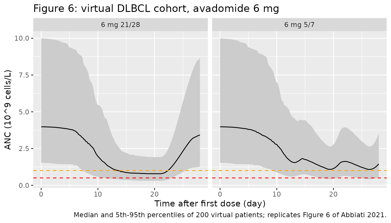
Figure 8: time of the ANC nadir
vp_sim |>
  dplyr::filter(grepl("^4 mg", treatment), time <= 28 * 24) |>
  group_by(treatment, sim.id) |>
  summarise(t_nadir = time[which.min(ANC)] / 24, .groups = "drop") |>
  group_by(treatment) |>
  summarise(
    p10 = quantile(t_nadir, 0.1), median = median(t_nadir), p90 = quantile(t_nadir, 0.9),
    .groups = "drop"
  ) |>
  dplyr::rename(
    "Regimen" = treatment,
    "10th pct (day)" = p10,
    "Median (day)" = median,
    "90th pct (day)" = p90
  ) |>
knitr::kable(digits = 1, caption = "Time of ANC nadir after the first dose, first cycle (4 mg).")| Regimen | 10th pct (day) | Median (day) | 90th pct (day) |
|---|---|---|---|
| 4 mg 14/28 | 14.0 | 14.2 | 14.8 |
| 4 mg 21/28 | 20.8 | 20.8 | 20.8 |
| 4 mg 28/28 | 23.8 | 25.8 | 27.8 |
| 4 mg 3/7 | 24.8 | 25.0 | 26.1 |
| 4 mg 5/7 | 26.2 | 26.2 | 26.3 |
| 4 mg 7/14 | 21.4 | 21.5 | 22.2 |
Figure 8 describes the nadir on the paper’s day scale, where the first dose is day 1, so each value here reads one day earlier. The nadir falls at the start of the last dosing holiday for 7/14 and 21/28: day 21 in the paper, days 20.8-21.5 after the first dose here. For 14/28 it falls around days 15-17 in the paper, about 14 days after the first dose here. On 28/28 it drifts late in the cycle. On 5/7, most patients reach their nadir in the final weekend (paper: ~91% at day 27; here ~26.2 days after the first dose). The paper also puts ~9% of 5/7 patients at day 20, which this cohort does not reproduce (see Assumptions).
Cohort comparison
ev_cmp <- rxode2::et(amt = 4, time = schedule_days(5, 7, 28) * 24, cmt = "depot") |>
  rxode2::et(seq(0, 28 * 24, by = 2))
lapply(list(GBM = mod_gbm, DLBCL = mod_dlbcl, MM = mod_mm), function(m) {
  as.data.frame(rxode2::rxSolve(m, events = ev_cmp, method = "cvode", atol = 1e-10, rtol = 1e-10))
}) |>
  bind_rows(.id = "cohort") |>
  ggplot(aes(time / 24, ANC, colour = cohort)) +
  geom_line() +
  labs(
    x = "Time after first dose (day)", y = "ANC (10^9 cells/L)",
    title = "Typical patient, 4 mg 5/7, baseline ANC 4.5 x 10^9/L",
    caption = "Table I parameter sets for GBM, DLBCL and MM."
  )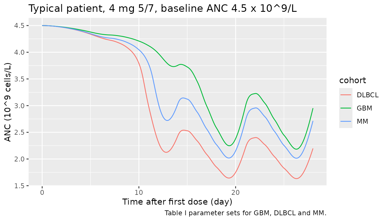
The DLBCL set has a smaller marrow reservoir, a weaker proliferative response and less capacity to push cells through the maturation block (lower gamma, reservoir ratio and KM fraction; Table I). It produces the deepest drop, which matches the authors’ reading of Table I.
Assumptions and deviations
- Central volume (V/F = 48.7 L) back-solved. The supplement prints the PK model only as micro-constants (k_abs, k12, k21, k_el, lag), and neither the paper nor the supplement gives a volume. The PK is cited to Cheng et al. 2021 (Clin Pharmacol Adv Appl 13:61-71). The constants are not that paper’s final model: Cheng reports ka = 4.14 1/h, a 0.246 h lag and a peripheral volume held at 10 L. So the volume cannot be carried from it. The authors deposited their simulated plasma profile for 5 mg on the 5/7 schedule (Supplementary file MOESM2, 40 doses, in ng/mL). With the printed rate constants, V/F = 48.70 L reproduces 97% of that profile’s points to within 0.5%, and the rest sit on the steep absorption upstrokes. It also reproduces every first-cycle AUC and Cmax in Table II (PK section above). The implied CL/F = 3.45 L/h is close to Cheng’s typical 3.63 L/h. The PK carries no between-subject variability, as in the paper (“population PK was not included”, Discussion).
- Table II AUC units. The AUC column is headed “ng/mlh”, but the deposited profile integrates to 1181 ng/mL x day over 28 days for the 5 mg 5/7 row (1181 in the table), i.e. 28,340 ngh/mL. The values are therefore in ng/mL x day. The Results text quotes the same numbers in”ng/ml*h” (1417 and 1515 for 6 mg 5/7 and 21/28).
- Table I derived-value typos. For DLBCL and MM, Table I prints Reserv0 = 1.25E10 cell/L, but the stated formula (2.5 x 4.5E9) gives 1.125E10. The printed kout (0.0092 1/h) and ktr4 (0.0256 1/h) follow from 1.125E10, so the model computes Reserv0 from the formula. For MM, Table I prints KM = 2.015E9 cell/L, while 0.45 x 4.5E9 = 2.025E9; the printed Vmax = 1.736E8 follows from 2.025E9. The model derives both from their formulas, so neither typo enters it.
- Cell units. The paper’s cells/L quantities are carried in 10^9 cells/L (ANC 4.5 rather than 4.5E9). The model is linear in the cell scale: KM and Vmax are defined relative to the baseline, and both feedbacks are ratios. The trajectories are therefore identical.
- Virtual population. The authors’ kernel-density estimates are not published. The virtual patients here are drawn from the Figure 4b histograms of the authors’ 1000-patient cohort, which the maintainers read exactly from the vector figure. Parameters are sampled independently, as in the paper. The cohort is 200 patients rather than 1000, so each Table II cell carries a few percentage points of Monte Carlo error.
- Endpoint window and sampling. The 7-day endpoints follow the profile to day 35 and use a 2-hour grid. The paper does not state its grid. Its example that a toxicity from day 27 must last “at least up to day 34.5” suggests a coarser one. Dosing continues into cycle 2 past day 28.
- Figure 3 inputs. Each panel’s baseline ANC was taken from the start of its plotted curve. The authors’ R script confirms this for the two panels it reproduces (GBM 5 mg 5/7, Circ0 = 7e9; DLBCL 5 mg 5/7, 4e9). The second “DLBCL 4mg 5/7” panel matches except in its weekend troughs, which the published curve dips about 10% lower than the simulation (1.27 vs 1.40 x 10^9/L). Its exact input is not stated; it probably corresponds to the separate 4-patient 4 mg 5/7 group in Figure 2.
- Figure 8. The ~9% of 5/7 patients whose nadir the paper places at day 20 do not appear in this cohort. Figure 8 does not state its dose; the table above uses 4 mg.
- Not modelled. G-CSF was out of scope (data after the first G-CSF dose were removed), and dexamethasone co-medication in MM is not represented. No efficacy model was developed; the authors used AUC as a surrogate.
-
Solver. The egress feedback exponent (beta = 20)
makes the system extremely stiff once the ANC falls well below baseline,
especially for patients with a high baseline ANC. The neutrophil
simulations here use the CVODE BDF solver
(
method = "cvode", atol = rtol = 1e-10). The default liblsoda solver fails for part of the cohort on the long-holiday and high-dose schedules (2% to half of the patients, depending on the tolerance), and gives the same answer (to ~1e-7) where it succeeds. - No residual error or IIV. The model was fitted by minimising a weighted sum of absolute normalised differences in Matlab (fminsearch). Variability is represented only by the virtual population, so the packaged models are deterministic.