Model and source
- Citation: Pohl O, Baron K, Riggs M, French J, Garcia R, Gotteland J-P. A model-based analysis to guide gonadotropin-releasing hormone receptor antagonist use for management of endometriosis. British Journal of Clinical Pharmacology. 2022;88(5):2359-2371. doi:10.1111/bcp.15171
- Description: Two-compartment population pharmacokinetic model for linzagolix, an oral gonadotropin-releasing hormone (GnRH) receptor antagonist developed for endometriosis, in healthy women and women with endometriosis (Pohl 2022). Sequential zero-order then first-order oral absorption; fixed allometric body-weight scaling on apparent clearance (0.75) and apparent central volume (1) with a 58 kg reference; a categorical non-Caucasian effect on apparent clearance; and a proportional residual error whose variance differs between the EDELWEISS phase 2b study and the phase 1 studies and additionally carries a subject-level random effect.
- Article: https://doi.org/10.1111/bcp.15171
- Supporting Information (open access, PMC9306723): https://pmc.ncbi.nlm.nih.gov/articles/PMC9306723/
Linzagolix (also known as OBE2109 / KLH2109) is an oral, non-peptide, selective gonadotropin-releasing hormone (GnRH) receptor antagonist developed for the management of endometriosis-associated pain. Pohl 2022 is an integrated model-informed dose-selection analysis: a population PK model feeds a PK- oestradiol (E2) model, which in turn drives statistical models of pelvic pain and uterine bleeding and a quantitative systems pharmacology model of lumbar spine bone mineral density.
This vignette validates the two structural pharmacology sub-models of the paper, packaged as two model files:
-
Pohl_2022_linzagolix– the population PK model (Table 4). -
Pohl_2022_linzagolix_e2– the PK-oestradiol exposure-response model (Table 5), driven by the daily AUC that the PK model generates.
The three remaining sub-models of the paper are statistical outcome models (pelvic pain, uterine bleeding) or a systems model whose structure is wholly inherited from an upstream publication (bone mineral density). Why each is not packaged here is set out under “Assumptions and deviations” below.
Population
The population PK analysis pooled 4250 linzagolix concentration observations from 756 women across five clinical trials (Table 1 and Table 3): the phase 1 first-in-human SAD/MAD study KLH1101 (12.5-400 mg single doses; 100-400 mg daily), the phase 2b dose-ranging study EDELWEISS (NCT02778399; placebo and 50-200 mg daily for 24 weeks in 330 women aged 18-45 with endometriosis), the clinical pharmacology studies 16-OBE2109-011 and 17-OBE2109-008 (100-200 mg daily for 42-70 days in healthy women, with and without hormonal add-back therapy), and KLH1204 (NCT02778919; placebo and 25-100 mg daily for 24 weeks in 440 Japanese women with endometriosis).
Approximately 24% of subjects and 55% of observations came from healthy volunteers; subjects receiving placebo contributed no records to the population PK analysis set. Median body weight ranged from 53.9 kg (KLH1204) to 65.5 kg (EDELWEISS) and median age from 32 to 40 years (Table 3). The proportion of Caucasian subjects ranged from 0% (KLH1204, KLH1201-1203) to 100% (17-OBE2109-008). Both Caucasian and non-Caucasian subjects were deliberately retained in the PK analysis to reduce parameter uncertainty, even though the dose-selection objective targeted a Caucasian/non-Asian population. About 5% of concentrations were below the quantitation limit and were dropped (Supporting Information section 1.1).
The same information is available programmatically via the model’s
population metadata
(readModelDb("Pohl_2022_linzagolix")()$population).
Source trace
The per-parameter origin is recorded as an in-file comment next to
each ini() entry in
inst/modeldb/specificDrugs/Pohl_2022_linzagolix.R. The
table below collects them in one place for review.
| Equation / parameter | Value | Source location |
|---|---|---|
| Two-compartment disposition with sequential zero-order then first-order oral absorption | n/a | Results section 3.1 (“2-compartment, linear PK model … using a sequential zero-order/first-order process”); Supporting Information section 3.1 |
lcl (CL/F) |
0.422 L/h | Table 4, “CL/F (L/h)”, 95% CI 0.393-0.455 |
lvc (V2/F) |
5.13 L | Table 4, “V2/F (L)”, 95% CI 4.19-6.18 |
lq (Q/F) |
0.168 L/h | Table 4, “Q/F (L/h)”, 95% CI 0.130-0.225 |
lvp (V3/F) |
3.12 L | Table 4, “V3/F (L)”, 95% CI 2.83-3.41 |
lka (KA) |
2.49 /h | Table 4, “KA”, 95% CI 2.04-3.08 |
ld1 (D1) |
0.644 h | Table 4, “D1 (h)”, 95% CI 0.314-1.24 |
e_wt_cl |
0.75 (fixed) | Table 4, “CL/F ~ (weight 58 kg)” = 0.75 FIXED; Supporting Information section 4.1 |
e_wt_vc |
1.00 (fixed) | Table 4, “V2/F ~ (weight 58 kg)” = 1.00 FIXED; Supporting Information section 4.1 |
e_nonwhite_cl |
0.08 | Table 4, “CL/F ~ non-Caucasian” ratio 1.08, 95% CI 1.05-1.12 |
etalcl |
0.0354 | Table 4, “IIV-CL/F”, shrinkage 16.5% |
etalvc |
0.0444 | Table 4, “IIV-V2/F”, shrinkage 62.0% |
etald1 |
0.510 | Table 4, “IIV-D1”, shrinkage 46.2% |
eta_re |
0.764 | Table 4, “IIV-sigma2” (subject-level random effect on the residual error variance), shrinkage 24.8% |
propSdEdelweiss |
sqrt(0.118) = 0.3435 | Table 4, “EDELWEISS data”, 95% CI 0.0698-0.206 |
propSdOther |
sqrt(0.0389) = 0.1972 | Table 4, “All other studies”, 95% CI 0.0309-0.0502 |
| Reference weight 58 kg | n/a | Table 4 covariate rows and Supporting Information section 4.1 |
| Validation target: steady-state AUC by dose | see below | Figure 2 (EDELWEISS, 50/75/100/200 mg) |
The PK-E2 model (Pohl_2022_linzagolix_e2) draws its
structure from the Supporting Information and its values from Table
5.
| Equation / parameter | Value | Source location |
|---|---|---|
Core PK-E2 equation
E2 = E2_0 * (1 - Imax*AUC^h/(AUC50^h + AUC^h)) * (BL_E2/52)^theta * (1 + PB)
|
n/a | Supporting Information section 3.2, display equation (stored in the
.docx as a raster image); Hill exponents restored, see
“Encoding decisions” below |
Baseline-E2 covariate equation
E2_0 = theta_BASE * (WT/58)^t5 * (AGE/35)^t6 * t7^ASIAN * exp(eta)
|
n/a | Supporting Information section 3.2 (CodeCogs-encoded display equation) |
theta_BASE patient / healthy switch |
n/a | Supporting Information section 3.2 (CodeCogs-encoded display equation) |
Placebo drift
PB = theta_ESS * (1 - exp(-theta_EK * WEEK))
|
n/a | Supporting Information section 3.2 (CodeCogs-encoded display equation) |
lbl_e2_patient |
59.1 pg/mL | Table 5, “Baseline E2, patients”, 95% CI 52.5-65.6 |
lbl_e2_healthy |
26.6 pg/mL | Table 5, “Baseline E2, healthy”, 95% CI 23.3-29.8 |
lauc50 |
1.68e5 ng*h/mL | Table 5, “Linzagolix AUC50”, 95% CI 1.44e5-1.91e5; Supporting Information section 4.2 |
lhill |
1.78 | Table 5, “Sigmoidicity parameter”, 95% CI 1.49-2.08; Supporting Information section 4.2 |
limax |
1 (fixed) | Not reported anywhere in the source; fixed by falsification against the paper’s own published outputs, see below |
e_wt_bl_e2 |
-0.699 | Table 5, “Baseline E2 ~ (weight 58 kg)”, 95% CI -0.958 to -0.441 |
e_age_bl_e2 |
0.0829 | Table 5, “Baseline E2 ~ (age 35 y)”, 95% CI -0.157 to 0.323 |
e_nonwhite_bl_e2 |
0.804 | Table 5, “Baseline E2 ~ non-Caucasian”, 95% CI 0.702-0.907 |
e_bl_e2_drug |
-0.120 | Table 5, “Baseline E2 ~ linzagolix drug effect”, 95% CI -0.212 to -0.0279 |
lemax_pbo |
0.65 | Table 5, “Placebo increase factor”, 95% CI 0.465-0.834; Supporting Information section 4.2 gives the same quantity as a 1.650-fold maximum increase |
lkp_e2 |
0.231 /week (fixed) | Table 5, “Placebo effect rate constant”, FIXED; Supporting Information section 3.2 |
e_abt_e2 |
1.58 pg/mL/week | Table 5, “E2 increase rate on add-back therapy”, 95% CI 0.990-2.16; functional form not printed by the source |
etalbl_e2 |
0.310 | Table 5, “IIV-baseline E2”, shrinkage 11.9% |
expSdPatient |
sqrt(0.610) = 0.78102 | Table 5, “Patients”, 95% CI 0.571-0.649 |
expSdHealthy |
sqrt(0.241) = 0.49092 | Table 5, “Healthy”, 95% CI 0.179-0.303 |
| Normalisation constants 52 pg/mL, 58 kg, 35 y | n/a | Supporting Information section 3.2 equations (the 52 pg/mL constant appears only inside the equation, in no table) |
| Validation target: week-24 E2 target window by dose | 20-50 pg/mL at 75-150 mg | Results section 3.3 |
A note on the signs in Table 5. Three Table 5
covariate estimates are negative, but the minus glyph is lost by every
text extraction of the PDF and of the JATS XML alike. The signs are
nonetheless unambiguous from the printed confidence intervals:
-0.699 is printed with the interval “0.958 to 0.441”, which
is only in ascending order if both bounds are negative, and the same
holds for -0.120 with “0.212 to 0.0279”. For
0.0829 the interval is printed “0.157 to 0.323”, and a
point estimate of 0.0829 cannot lie below a lower bound of 0.157 – so
that bound is -0.157 and the estimate itself is positive.
The narrative agrees, describing “a modest inverse relationship between
weight and baseline E2”.
Virtual cohort
Original observed data are not publicly available. The cohort below approximates the EDELWEISS phase 2b population (Table 3: median weight 65.5 kg, 94% Caucasian, median age 32 years), which is the population shown in Figure 2 of the paper, and doses it at the four fixed dose levels that figure reports.
Body weight is drawn log-normally with a median of 65.5 kg and a spread giving roughly the 17.8 kg standard deviation reported in Table 3. Age is not a covariate in the population PK model and is therefore not simulated.
# `set.seed()` seeds R's RNG. It does NOT seed rxode2's simulation RNG, and
# rxode2's streams are partitioned PER SOLVER THREAD -- so the cohort below is
# reproducible on this machine and different on a machine with a different
# thread count. Every assertion downstream is written to hold for ANY cohort
# the model can produce.
set.seed(20220401)

n_per_arm <- 200L
doses_mg <- c(50, 75, 100, 200)

tau <- 24        # dosing interval (h)
n_doses <- 10L   # 10 daily doses; terminal half-life is ~13 h so steady state
                 # is effectively complete well before the final interval
t_last <- tau * (n_doses - 1L)   # time of the final dose = 216 h

# Observation grid: coarse over the whole treatment period for the profile
# plot, dense over the final (steady-state) dosing interval for NCA.
obs_times <- sort(unique(c(
  seq(0, t_last, by = 4),
  seq(t_last, t_last + tau, by = 0.5)
)))

make_cohort <- function(n, dose_mg, id_offset = 0L) {
  subj <- tibble(
    id = id_offset + seq_len(n),
    # Table 3, EDELWEISS: weight median 65.5 kg (SD 17.8 kg).
    WT = 65.5 * exp(stats::rnorm(n, mean = 0, sd = 0.26)),
    # Table 3, EDELWEISS: 94% Caucasian.
    RACE_WHITE = stats::rbinom(n, size = 1, prob = 0.94),
    # These subjects are simulated as EDELWEISS records, so the EDELWEISS
    # residual-error magnitude applies.
    STUDY_EDELWEISS = 1,
    dose_group = paste0(dose_mg, " mg")
  )

  dosing <- subj |>
    tidyr::crossing(time = tau * seq(0, n_doses - 1L)) |>
    mutate(
      amt = dose_mg,
      evid = 1L,
      # cmt is the ODE state receiving the dose; rate = -2 tells rxode2 to use
      # the modelled zero-order duration dur(depot) <- d1.
      cmt = "depot",
      rate = -2
    )

  obs <- subj |>
    tidyr::crossing(time = obs_times) |>
    mutate(
      amt = NA_real_,
      evid = 0L,
      # The ODE state, never the algebraic observable name "Cc".
      cmt = "central",
      rate = 0
    )

  bind_rows(dosing, obs) |> arrange(id, time, desc(evid))
}

events <- bind_rows(lapply(seq_along(doses_mg), function(i) {
  make_cohort(n_per_arm, doses_mg[i], id_offset = (i - 1L) * n_per_arm)
}))

# Disjoint IDs across arms are mandatory: duplicate ids silently merge into a
# single subject receiving the summed dose.
stopifnot(!anyDuplicated(unique(events[, c("id", "time", "evid")])))
stopifnot(dplyr::n_distinct(events$id) == n_per_arm * length(doses_mg))
Simulation
mod <- readModelDb("Pohl_2022_linzagolix")

sim <- rxode2::rxSolve(
  mod,
  events = events,
  keep = c("dose_group", "WT", "RACE_WHITE", "STUDY_EDELWEISS")
) |>
  as.data.frame()
#> ℹ parameter labels from comments will be replaced by 'label()'

# `cl` is a model-computed variable, so rxode2 returns it per row. It is the
# individual apparent clearance actually used by the solver, which the exact
# steady-state mass-balance check below relies on.
stopifnot(all(c("Cc", "cl") %in% names(sim)))
stopifnot(all(sim$Cc >= 0))
sim |>
  filter(time <= t_last + tau) |>
  group_by(dose_group, time) |>
  summarise(
    Q05 = quantile(Cc, 0.05),
    Q50 = quantile(Cc, 0.50),
    Q95 = quantile(Cc, 0.95),
    .groups = "drop"
  ) |>
  mutate(dose_group = factor(dose_group, levels = paste0(doses_mg, " mg"))) |>
  ggplot(aes(time / 24, Q50)) +
  geom_ribbon(aes(ymin = Q05, ymax = Q95), alpha = 0.25) +
  geom_line() +
  facet_wrap(~dose_group) +
  labs(
    x = "Time (days)", y = "Linzagolix concentration (ug/mL)",
    title = "Simulated linzagolix concentration-time profiles",
    caption = "Median and 5th-95th percentile band, 200 subjects per dose arm."
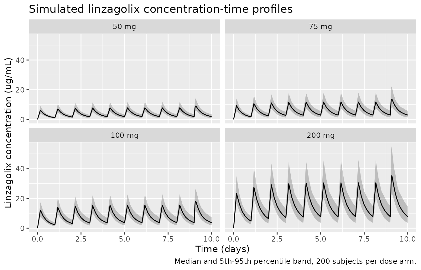
  )
PKNCA validation
NCA is computed over the final dosing interval (216-240 h), which is at steady state.
sim_nca <- sim |>
  dplyr::filter(!is.na(Cc)) |>
  dplyr::select(id, time, Cc, dose_group)

# Guarantee a time-zero row per (id, dose_group). Linzagolix is given orally,
# so the pre-dose concentration is zero.
sim_nca <- dplyr::bind_rows(
  sim_nca,
  sim_nca |> dplyr::distinct(id, dose_group) |> dplyr::mutate(time = 0, Cc = 0)
) |>
  dplyr::distinct(id, dose_group, time, .keep_all = TRUE) |>
  dplyr::arrange(id, dose_group, time)

conc_obj <- PKNCA::PKNCAconc(
  sim_nca, Cc ~ time | dose_group + id,
  concu = "ug/mL", timeu = "h"
)

dose_df <- events |>
  dplyr::filter(evid == 1) |>
  dplyr::select(id, time, amt, dose_group)

dose_obj <- PKNCA::PKNCAdose(dose_df, amt ~ time | dose_group + id, doseu = "mg")

intervals <- data.frame(
  start   = t_last,
  end     = t_last + tau,
  cmax    = TRUE,
  tmax    = TRUE,
  cmin    = TRUE,
  cav     = TRUE,
  auclast = TRUE
)

nca_res <- PKNCA::pk.nca(PKNCA::PKNCAdata(conc_obj, dose_obj, intervals = intervals))

nca_wide <- as.data.frame(nca_res) |>
  dplyr::select(dose_group, id, PPTESTCD, PPORRES) |>
  tidyr::pivot_wider(names_from = PPTESTCD, values_from = PPORRES)

stopifnot(nrow(nca_wide) == n_per_arm * length(doses_mg))
stopifnot(!anyNA(nca_wide$auclast))
Exact steady-state mass balance
At steady state the area under the curve over one dosing interval is
exactly Dose / CL. Both sides of this comparison use the
same drawn individual clearance, so the only sources of
disagreement are trapezoidal integration error on the absorption peak
and the small amount of accumulation still outstanding after 10 doses. A
tight bound is therefore the correct assertion here (unlike a
cohort-extreme comparison, which would not be reproducible across rxode2
builds).
cl_by_id <- sim |>
  dplyr::group_by(id, dose_group) |>
  dplyr::summarise(cl = dplyr::first(cl), .groups = "drop")

dose_by_id <- dose_df |>
  dplyr::group_by(id) |>
  dplyr::summarise(amt = dplyr::first(amt), .groups = "drop")

mb <- nca_wide |>
  dplyr::left_join(cl_by_id, by = c("id", "dose_group")) |>
  dplyr::left_join(dose_by_id, by = "id") |>
  dplyr::mutate(
    auc_expected = amt / cl,
    pct_diff = 100 * (auclast - auc_expected) / auc_expected
  )

mb_summary <- mb |>
  dplyr::group_by(dose_group) |>
  dplyr::summarise(
    `Median AUC0-tau (ug*h/mL)` = median(auclast),
    `Median Dose/CL (ug*h/mL)` = median(auc_expected),
    `Median % difference` = median(pct_diff),
    `90th pctile |% difference|` = quantile(abs(pct_diff), 0.9),
    .groups = "drop"
  )

knitr::kable(
  mb_summary, digits = 2,
  caption = "Steady-state AUC0-tau from PKNCA vs the exact identity Dose / CL."
)| dose_group | Median AUC0-tau (ug*h/mL) | Median Dose/CL (ug*h/mL) | Median % difference | 90th pctile |% difference| |
|---|---|---|---|---|
| 100 mg | 210.64 | 210.77 | -0.05 | 0.17 |
| 200 mg | 430.03 | 430.12 | -0.04 | 0.13 |
| 50 mg | 108.82 | 108.91 | -0.05 | 0.13 |
| 75 mg | 164.99 | 165.07 | -0.05 | 0.12 |
Dose proportionality
The model is linear, so steady-state exposure must scale exactly with dose.
auc_med <- mb |>
  dplyr::group_by(dose_group) |>
  dplyr::summarise(auc = median(auclast), .groups = "drop")

ratio_200_50 <- auc_med$auc[auc_med$dose_group == "200 mg"] /
  auc_med$auc[auc_med$dose_group == "50 mg"]

ratio_100_50 <- auc_med$auc[auc_med$dose_group == "100 mg"] /
  auc_med$auc[auc_med$dose_group == "50 mg"]

# Guard against a lookup that silently matched nothing (a gate that cannot
# go red is worse than no gate).
stopifnot(length(ratio_200_50) == 1L, length(ratio_100_50) == 1L)

c(`200 mg / 50 mg` = ratio_200_50, `100 mg / 50 mg` = ratio_100_50)
#> 200 mg / 50 mg 100 mg / 50 mg
#>       3.951709       1.935661

stopifnot(
  abs(ratio_200_50 - 4) < 0.4,
  abs(ratio_100_50 - 2) < 0.2
)
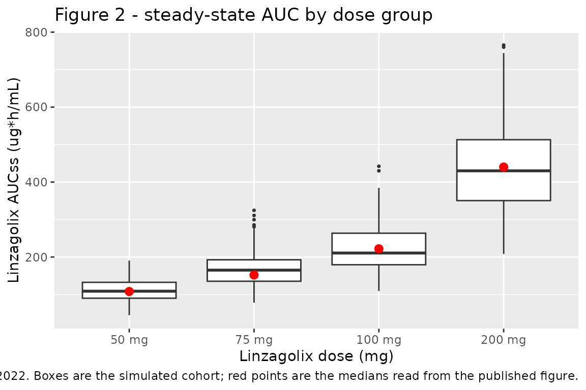
Comparison against the published steady-state exposures (Figure 2)
Pohl 2022 reports no NCA table. The only published exposure summary
is Figure 2, a box-and-whisker plot (the caption calls them histograms)
of model-based steady-state AUC by EDELWEISS dose group, on a
ug h/mL axis. The reference values below were read off that
figure’s medians and are therefore approximate – they are digitised
comparison targets, not published point estimates, and are flagged as
such under “Assumptions and deviations”.
# Medians read from Figure 2 of Pohl 2022 (ug*h/mL). Digitised, +/- ~5%.
published <- tibble::tribble(
  ~dose_group, ~auclast,
  "50 mg",     108,
  "75 mg",     152,
  "100 mg",    222,
  "200 mg",    440
)

cmp <- nlmixr2lib::ncaComparisonTable(
  simulated = nca_res,
  reference = published,
  by        = "dose_group",
  params    = "auclast",
  units     = c(auclast = "ug*h/mL"),
  tolerance_pct = 20
)

knitr::kable(
  cmp,
  caption = paste(
    "Simulated steady-state AUC0-tau vs medians read from Figure 2 of",
    "Pohl 2022. * differs from the reference by >20%."
  )
)| NCA parameter | dose_group | Reference | Simulated | % diff |
|---|---|---|---|---|
| AUClast (ug*h/mL) | 50 mg | 108 | 109 | +0.8% |
| AUClast (ug*h/mL) | 75 mg | 152 | 165 | +8.5% |
| AUClast (ug*h/mL) | 100 mg | 222 | 211 | -5.1% |
| AUClast (ug*h/mL) | 200 mg | 440 | 430 | -2.3% |
# Replicates Figure 2 of Pohl 2022: distribution of model-based steady-state
# AUC by linzagolix dose group.
mb |>
  mutate(dose_group = factor(dose_group, levels = paste0(doses_mg, " mg"))) |>
  ggplot(aes(dose_group, auclast)) +
  geom_boxplot(outlier.size = 0.6) +
  geom_point(
    data = published |>
      mutate(dose_group = factor(dose_group, levels = paste0(doses_mg, " mg"))),
    aes(dose_group, auclast), colour = "red", size = 2.5
  ) +
  labs(
    x = "Linzagolix dose (mg)", y = "Linzagolix AUCss (ug*h/mL)",
    title = "Figure 2 - steady-state AUC by dose group",
    caption = paste(
      "Replicates Figure 2 of Pohl 2022. Boxes are the simulated cohort;",
      "red points are the medians read from the published figure."
    )
  )
nca_wide |>
  dplyr::group_by(dose_group) |>
  dplyr::summarise(
    cmax = median(cmax), tmax = median(tmax), cmin = median(cmin),
    cav = median(cav), auclast = median(auclast), .groups = "drop"
  ) |>
  dplyr::rename(
    "Dose group" = dose_group,
    "Cmax,ss (ug/mL)" = cmax,
    "Tmax (h)" = tmax,
    "Cmin,ss (ug/mL)" = cmin,
    "Cav,ss (ug/mL)" = cav,
    "AUC0-tau (ug*h/mL)" = auclast
  ) |>
  knitr::kable(
    digits = 2,
    caption = "Median simulated steady-state NCA parameters by dose group."
)| Dose group | Cmax,ss (ug/mL) | Tmax (h) | Cmin,ss (ug/mL) | Cav,ss (ug/mL) | AUC0-tau (ug*h/mL) |
|---|---|---|---|---|---|
| 100 mg | 18.40 | 1.5 | 3.70 | 8.78 | 210.64 |
| 200 mg | 36.30 | 1.5 | 7.77 | 17.92 | 430.03 |
| 50 mg | 9.27 | 1.5 | 1.97 | 4.53 | 108.82 |
| 75 mg | 13.90 | 1.5 | 2.98 | 6.87 | 164.99 |
PK-oestradiol model
The PK-E2 model takes the daily linzagolix AUC as its exposure driver
(AUC_LZGX, in ng*h/mL) and returns serum
oestradiol in pg/mL. The two models are chained exactly as
the authors chained them: the PK model of Table 4 generates the
individual daily AUC, which the E2 model of Table 5 consumes. Because
linzagolix has linear PK and a roughly 8 h half-life, the steady-state
daily AUC under once-daily dosing is Dose / (CL/F) – the
quantity whose distribution the paper plots in Figure 2.
mod_e2 <- rxode2::rxode(readModelDb("Pohl_2022_linzagolix_e2"))
#> ℹ parameter labels from comments will be replaced by 'label()'

# Typical-value (zeroRe) solve: the paper's dose-selection simulations describe
# a *reference* Caucasian patient, so the replication below must be a
# typical-value solve, not a random cohort.
mod_e2_tv <- rxode2::zeroRe(mod_e2)
#> Warning: No sigma parameters in the model

# Reference Caucasian endometriosis patient of the dose-selection analysis.
# Weight 65 kg is stated in Supporting Information section 4.3; age and
# baseline E2 are the EDELWEISS medians of Table 3.
ref_wt    <- 65
ref_age   <- 32
ref_bl_e2 <- 53.0

# Individual CL/F from the companion PK model (Table 4), Caucasian.
ref_cl <- 0.422 * (ref_wt / 58)^0.75
Reproducing the paper’s stated target-dose window
Section 3.3 of the paper makes a precise, quantitative claim: “Doses between 75 and 150 mg daily were associated with week 24 E2 concentrations in the proposed target window of 20-50 pg/mL.” That single sentence constrains the model at both edges of the window, and is the strongest available check on the extraction, because the paper publishes no E2 parameter table other than the one the model was built from.
doses_e2 <- c(25, 50, 75, 100, 125, 150, 200)

e2_events <- rxode2::et(seq(0, 24 * 7 * 24, by = 24)) |>
  rxode2::et(id = seq_along(doses_e2))

e2_dat <- as.data.frame(e2_events)
# AUC in ng*h/mL: the PK model's concentrations are ug/mL, so the ug*h/mL
# steady-state integral Dose/CL is multiplied by 1000.
e2_dat$AUC_LZGX    <- (doses_e2 / ref_cl * 1000)[e2_dat$id]
e2_dat$WT          <- ref_wt
e2_dat$AGE         <- ref_age
e2_dat$BL_E2       <- ref_bl_e2
e2_dat$RACE_WHITE  <- 1
e2_dat$DIS_HEALTHY <- 0
e2_dat$T_ABT       <- 0

e2_sol <- rxode2::rxSolve(mod_e2_tv, e2_dat, returnType = "data.frame")
#> ℹ omega/sigma items treated as zero: 'etalbl_e2'
#> Warning: multi-subject simulation without without 'omega'

wk24 <- e2_sol[abs(e2_sol$time - 24 * 7 * 24) < 1e-6, c("id", "e2")]
wk24$dose <- doses_e2[wk24$id]
wk24$in_window <- wk24$e2 >= 20 & wk24$e2 <= 50

wk24 |>
  dplyr::transmute(
    "Daily dose (mg)"    = dose,
    "Week-24 E2 (pg/mL)" = round(e2, 1),
    "In 20-50 pg/mL"     = ifelse(in_window, "yes", "no")
  ) |>
  knitr::kable(
    caption = paste(
      "Week-24 oestradiol for the Caucasian reference patient.",
      "The paper states that doses of 75-150 mg -- and only those --",
      "fall inside the 20-50 pg/mL target window."
    )
)| Daily dose (mg) | Week-24 E2 (pg/mL) | In 20-50 pg/mL | |
|---|---|---|---|
| 169 | 25 | 78.5 | no |
| 338 | 50 | 60.9 | no |
| 507 | 75 | 45.7 | yes |
| 676 | 100 | 34.5 | yes |
| 845 | 125 | 26.5 | yes |
| 1014 | 150 | 20.9 | yes |
| 1183 | 200 | 13.8 | no |
# The paper's claim, asserted exactly: 75-150 mg inside, 50 and 200 mg outside.
# This is a typical-value solve with no random effects, so the result is
# deterministic across machines and rxode2 versions and a hard assertion is
# correct here (contrast a cohort-extreme assertion).
inside  <- wk24$dose[wk24$in_window]
stopifnot(
  identical(sort(inside), c(75, 100, 125, 150)),
  !wk24$in_window[wk24$dose == 50],
  !wk24$in_window[wk24$dose == 200]
)
Falsifying the two unprinted elements of the published equation
The Supporting Information equation, recovered from the raster image
it is stored as, contains neither a Hill exponent nor a value for
theta_IMAX – yet Table 5 reports a sigmoidicity parameter
of 1.78, and both the main text and Supporting Information section 3.2
describe “a sigmoid inhibitory Emax model”. Rather than guess, the two
candidates are tested against the paper’s own published output
above.
# Re-derive week-24 E2 under the alternatives, by hand from Table 5, so the
# comparison does not depend on the packaged model file.
e2_at <- function(dose, imax, hill) {
  auc   <- dose / ref_cl * 1000
  auc50 <- 1.68e5
  e2_0  <- 59.1 * (ref_wt / 58)^(-0.699) * (ref_age / 35)^0.0829
  pb24  <- 0.65 * (1 - exp(-0.231 * 24))
  e2_0 * (1 - imax * auc^hill / (auc50^hill + auc^hill)) *
    (ref_bl_e2 / 52)^(-0.120) * (1 + pb24)
}

falsify <- data.frame(dose = doses_e2)
falsify$as_packaged  <- e2_at(falsify$dose, imax = 1.0, hill = 1.78)
falsify$no_hill      <- e2_at(falsify$dose, imax = 1.0, hill = 1.00)
falsify$imax_0_9     <- e2_at(falsify$dose, imax = 0.9, hill = 1.78)

in_win <- function(x) ifelse(x >= 20 & x <= 50, "IN", "out")
falsify |>
  dplyr::transmute(
    "Daily dose (mg)"                    = dose,
    "Imax=1, Hill=1.78 (packaged)"       = paste0(round(as_packaged, 1), " ", in_win(as_packaged)),
    "Imax=1, no Hill"                    = paste0(round(no_hill, 1),     " ", in_win(no_hill)),
    "Imax=0.9, Hill=1.78"                = paste0(round(imax_0_9, 1),    " ", in_win(imax_0_9))
  ) |>
  knitr::kable(
    caption = paste(
      "Falsification of the alternatives. Only the packaged structure places",
      "75-150 mg inside the published target window and 200 mg outside it."
    )
)| Daily dose (mg) | Imax=1, Hill=1.78 (packaged) | Imax=1, no Hill | Imax=0.9, Hill=1.78 |
|---|---|---|---|
| 25 | 78.5 out | 67.3 out | 79.6 out |
| 50 | 60.9 out | 54 out | 63.7 out |
| 75 | 45.7 IN | 45.2 IN | 50 out |
| 100 | 34.5 IN | 38.8 IN | 39.9 IN |
| 125 | 26.5 IN | 34 IN | 32.8 IN |
| 150 | 20.9 IN | 30.3 IN | 27.7 IN |
| 200 | 13.8 out | 24.8 IN | 21.3 IN |
# Both alternatives put 200 mg INSIDE the window, contradicting the paper's
# own stated 150 mg upper bound. That is what rules them out.
stopifnot(
  in_win(falsify$no_hill[falsify$dose == 200])  == "IN",
  in_win(falsify$imax_0_9[falsify$dose == 200]) == "IN",
  in_win(falsify$as_packaged[falsify$dose == 200]) == "out"
)
The packaged structure also agrees with the model-based week-24 oestradiol medians shown in Figure 4 of the paper, which pools the EDELWEISS (Caucasian) and KLH1204 (Japanese) cohorts.
Oestradiol time course and the placebo drift
e2_sol$dose <- doses_e2[e2_sol$id]
e2_sol$week <- e2_sol$time / (24 * 7)

ggplot2::ggplot(
  e2_sol,
  ggplot2::aes(week, e2, colour = factor(dose), group = dose)
) +
  ggplot2::annotate(
    "rect", xmin = -Inf, xmax = Inf, ymin = 20, ymax = 50,
    fill = "grey80", alpha = 0.5
  ) +
  ggplot2::geom_line(linewidth = 0.8) +
  ggplot2::labs(
    x = "Week", y = "Oestradiol (pg/mL)", colour = "Dose (mg)",
    title = "Typical-value oestradiol time course by linzagolix dose",
    subtitle = "Shaded band is the 20-50 pg/mL target window of Pohl 2022"
  ) +
  ggplot2::theme_bw()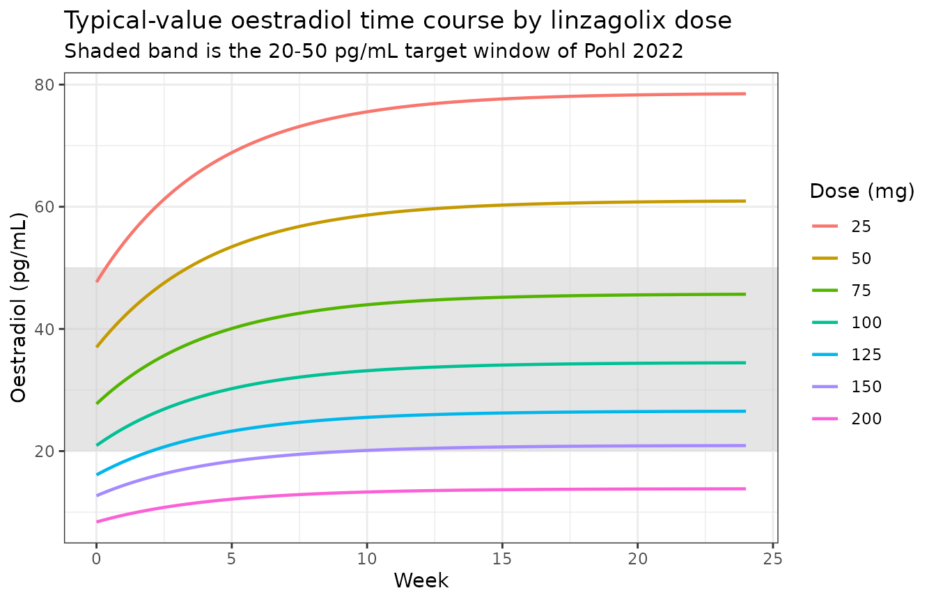
The upward drift visible in every arm is the model’s apparent placebo effect. Treatment started at menses, the nadir of the menstrual oestradiol cycle, so oestradiol appears to rise as cycle synchronisation is lost across the trial (Supporting Information section 3.2). The source fixed its rate constant so that the increase is essentially complete by week 12.
# The placebo state must reproduce PB(t) = 0.65 * (1 - exp(-0.231 * week))
# exactly, and be ~94% of its maximum at week 12 -- the source's stated reason
# for fixing the rate constant. Deterministic, so assert tightly.
pb <- e2_sol[e2_sol$id == 1, c("week", "e2_placebo")]
pb$closed_form <- 0.65 * (1 - exp(-0.231 * pb$week))

stopifnot(
  max(abs(pb$e2_placebo - pb$closed_form)) < 1e-6,
  abs(pb$closed_form[which.min(abs(pb$week - 12))] / 0.65 - 0.9375) < 0.01
)

cat(sprintf(
  "Placebo drift: max |ODE - closed form| = %.2e; %.1f%% of maximum at week 12.\n",
  max(abs(pb$e2_placebo - pb$closed_form)),
  100 * pb$closed_form[which.min(abs(pb$week - 12))] / 0.65
))
#> Placebo drift: max |ODE - closed form| = 2.19e-08; 93.7% of maximum at week 12.
Patient versus healthy-volunteer baseline
The source reports “approximately 2-fold higher baseline E2 in Caucasian patients relative to Caucasian HVs” (Results section 3.1).
bl_dat <- e2_dat[e2_dat$id == 1, ]
bl_dat$AUC_LZGX <- 0            # no drug: isolates the baseline term
bl_pair <- do.call(rbind, lapply(c(0, 1), function(h) {
  d <- bl_dat
  d$DIS_HEALTHY <- h
  s <- rxode2::rxSolve(mod_e2_tv, d, returnType = "data.frame")
  data.frame(healthy = h, e2_t0 = s$e2[s$time == 0])
}))
#> ℹ omega/sigma items treated as zero: 'etalbl_e2'
#> ℹ omega/sigma items treated as zero: 'etalbl_e2'

ratio <- bl_pair$e2_t0[bl_pair$healthy == 0] / bl_pair$e2_t0[bl_pair$healthy == 1]
stopifnot(abs(ratio - 59.1 / 26.6) < 1e-6)   # the Table 5 ratio, exactly
cat(sprintf(
  "Patient / healthy-volunteer baseline E2 ratio = %.2f (Table 5: 59.1 / 26.6 = %.2f).\n",
  ratio, 59.1 / 26.6
))
#> Patient / healthy-volunteer baseline E2 ratio = 2.22 (Table 5: 59.1 / 26.6 = 2.22).
Assumptions and deviations
Scope of this extraction
Pohl 2022 develops five linked sub-models. The two structural pharmacology models are packaged here; the three outcome / systems models are not, for the source-side reasons given below.
-
Population PK (Table 4) – packaged as
Pohl_2022_linzagolix, validated above. -
PK-E2 model (Table 5) – packaged as
Pohl_2022_linzagolix_e2, validated above. Two elements of the published equation had to be reconstructed; both are falsified against the paper’s own outputs rather than assumed, and are documented under “Encoding decisions within the PK-E2 model” below. -
Dysmenorrhoea and non-menstrual pelvic pain (Table
6) – repeated-measures logistic regressions of monthly
responder status on E2, fitted with
glmer. Logistic exposure-response models are in scope for this library, but this pair is not yet packaged for two source-side reasons. First, Table 6 reports odds ratios without the covariate centring constants needed to reconstruct the linear predictor: the intercept is given as an odds (6.27 for DYS, 0.326 for NMPP) but the paper never states the covariate values at which it applies, and a per-kilogram weight odds ratio is meaningless without its centring weight. Second, the NMPP column as published is not self-consistent: it repeats 0.987 for three different covariates (baseline pain, days 113-140, and E2) and 0.326 for two (intercept and days 141-168), reports a per-kilogram weight odds ratio of 5.94 (95% CI 3.57-8.31), and gives a baseline-pain odds ratio of 0.987 where the Supporting Information (section 4.3) states 4.5 (95% CI 2.73-6.28) for what appears to be the same quantity. Figure 8 supplies the fitted probability-vs-E2 curves for a defined reference patient and could in principle pin the centring, but resolving a published table against a digitised figure is a decision for the maintainers rather than a silent reconstruction. - Uterine bleeding (Table 7) – a repeated-measures zero-inflated Beta regression on the proportion of bleeding days in each 28-day interval, fitted in a GAMLSS framework with separate mean, dispersion and probability-of-zero submodels. Not yet packaged: nlmixr2 has no zero-inflated Beta likelihood, so replicating the authors’ structure would require either a new likelihood or a reformulation that is no longer the model they fitted. Table 7 also shares Table 6’s missing-centring problem, and repeats 0.683 for both the probability-of-zero intercept and its E2 coefficient.
-
Lumbar spine BMD (Table 8) – a quantitative systems
pharmacology model. Pohl 2022 estimated only the two parameters of the
E2 scaling function (E2-50 = 0.202 pg/mL, sigmoidicity 1.17) and fixed
all structural parameters to Riggs 2012 (CPT
Pharmacometrics Syst Pharmacol 1:e11, doi:10.1038/psp.2012.10),
which in turn fixes its own system parameters to Peterson & Riggs
2010 and the authors’
OpenBoneMincode deposit (https://github.com/metrumresearchgroup/OpenBoneMin). Both upstream sources were available when this model was built, but the underlying bone model is a 43-state, multi-hundred-parameter calcium/bone homeostasis system whose compartments have no canonical names in the library, and the published Riggs 2012 estimate of one power parameter (theta TGF-beta,latent = 0.075) disagrees with the corresponding constant in the code deposit (tgfbGAM = 0.0374). Because essentially the entire structure belongs to Riggs 2012 rather than to Pohl 2022 – which contributes only the two E2-scaling parameters of Table 8 – the bone model is properly a separate extraction of Riggs 2012 itself, not a sub-model of this paper. The Riggs 2012 paper was already available to the maintainers when this model was built, so it can be taken up as its own extraction.
Encoding decisions within the population PK model
-
Units. Doses are in mg and volumes in litres, so
Cc = central / vcis in mg/L, i.e.ug/mL. This matches the axis of Figure 2 (ug h/mL) and is consistent with Table 5’s AUC-50 of 1.68e5ng h/mL= 168ug h/mL. -
KA units. Table 4 lists KA with units “L/h”. KA is
a first-order absorption rate constant, so this is a typographical slip
in the source; the value 2.49 is used as
1/h. -
IIV and residual values are variances. Table 4
reports the interindividual terms as 0.0354 / 0.0444 / 0.510 / 0.764 and
the residual terms as 0.118 / 0.0389, which are NONMEM
$OMEGA/$SIGMAvariances (as variances they correspond to plausible CVs of 19% on CL/F and 34%/20% proportional error; read as standard deviations the residual error would be an implausible 3.9% for the phase 1 studies). The residual SDs in the model file are therefore the square roots of the tabulated values. -
Subject-level random effect on the residual
variance. Table 4’s “IIV-sigma2” is described in the Supporting
Information (section 3.1) as “a subject-level random effect on the
residual error variance”. It is implemented as a multiplier
exp(eta_re / 2)on the residual standard deviation, which is the correct transformation if the random effect acts on the variance as the label states. If the source instead placed the random effect on the standard deviation, the multiplier would beexp(eta_re); the paper does not print the NONMEM$ERRORblock, so this reading follows the printed label. -
Race reference category. Caucasian is the
typical-value reference, so the 8% clearance increase is applied on
(1 - RACE_WHITE). This matches the orientation used byHu_2014_bapineuzumab. - Weight effects. Only CL/F and V2/F carry the weight effect, with exponents fixed at 0.75 and 1 respectively and a 58 kg reference. Q/F and V3/F carry no covariate in the final model, so none is added.
- Add-back therapy. Studies 16-OBE2109-011 and 17-OBE2109-008 administered oestradiol/norethisterone add-back therapy. It affects the E2 model (Table 5) but no linzagolix PK parameter in Table 4, so it does not appear in this model.
Encoding decisions within the PK-E2 model
-
The Hill exponent is restored to the published
equation. The Supporting Information display equation (stored
in the
.docxas a raster image, which is why it survives no text extraction) prints the inhibitory term astheta_IMAX * AUC / (theta_AUC50 + AUC)– with no exponent anywhere. Table 5 nonetheless reports a “Sigmoidicity parameter” of 1.78, Supporting Information section 4.2 repeats it, and both the main text and Supporting Information section 3.2 describe “a sigmoid inhibitory Emax model”. The exponent is therefore placed in its standard position on both AUC terms. The vignette section “Falsifying the two unprinted elements” shows that dropping it (Hill = 1) contradicts the paper’s own statement that only 75-150 mg fall inside the 20-50 pg/mL window – without the exponent, 200 mg lands inside it. -
Imax is fixed to 1, and is not reported by the source at
all. Table 5 lists every other structural parameter,
including one explicitly marked FIXED, but carries no Imax row;
the equation carries a
theta_IMAXsymbol with no accompanying estimate. Complete suppression is both the mechanistically expected value for a GnRH receptor antagonist and, as the same falsification table shows, the only value consistent with the paper’s published dose window: at Imax = 0.9, 200 mg again falls inside it. This is the one parameter in either model file whose value is not taken from a printed number, and it is encoded asfixed()so that status is visible. -
The baseline-E2 exponent multiplies the whole
expression. Table 5 labels
-0.120as “Baseline E2 ~ linzagolix drug effect” and Supporting Information section 3.2 says “the linzagolix drug effect was assumed to be related to observed baseline E2 by an estimated exponent”, which reads as though the term belongs inside the inhibition bracket. The printed equation places(E2_BASE / 52)^thetaoutside it, multiplying the entire right-hand side, and the equation is followed here per the standing rule that a printed equation outranks prose. The numerical difference is small (the factor is 0.998 at the EDELWEISS median baseline). -
Add-back therapy: value published, functional form
not. Table 5 reports an “E2 increase rate on add-back therapy”
of 1.58 pg/mL/week, but the term appears in no printed equation. It is
encoded as an additive linear-in-time increment
e_abt_e2 * T_ABT, the only form consistent with the published pg/mL/week unit.T_ABTdefaults to 0, which is the entire EDELWEISS population and the whole dose-selection analysis, so every result in this vignette is independent of this choice. -
IIV and residual values are variances, on the same
NONMEM
$OMEGA/$SIGMAreading applied to Table 4, and for consistency with it: both tables use the same layout, and Table 4’s must be variances. The residual SDs in the model file are thereforesqrt(0.610)andsqrt(0.241). -
Log-transform-both-sides residual error. Supporting
Information section 3.2 states the model was “estimated using a
log-transform both sides approach with additive residual error with
respect to natural-logarithm transformed E2”, which is
~ lnorm()in nlmixr2 rather than~ prop(). -
The placebo drift is carried as a state.
PB(t) = theta_ESS * (1 - exp(-theta_EK * t))is encoded as the equivalent first-order approach-to-plateau ODE rather than as an explicit function oft. The vignette asserts agreement with the closed form to1e-6. Supporting Information section 4.2 independently confirms the(1 + PB)form of the main equation by quoting the same quantity as a “1.650-fold” maximum increase, i.e.1 + 0.65. -
Two convention warnings, accepted deliberately.
checkModelConventions()flags this model twice, both times for the same underlying reason: the library’s compartment register (inst/references/compartment-names.md) has no oestradiol entry.- The single-output observation variable
e2is not canonical.Ccis reserved for drug concentrations and would be wrong here – oestradiol is an endogenous hormone, not linzagolix. The register does already carry a family of bare hormone-biomarker PD outputs (pth,shbg,prolactin,insulin,igf1,glp1,t3_serum/t4_serum/tsh_serum), of whiche2would be a well-formed member. - The state
e2_placebois not canonical, for the same reason. The register likewise already carries the<biomarker>_placebodrift-state suffix (fpg_placebo,hba1c_placebo, alongsidefpg_drugandhba1c_drug), of whiche2_placebowould be a well-formed member.
buildModelDb()builds the model and the registry cleanly. - The single-output observation variable
Simulation assumptions
- The virtual cohort’s body-weight distribution (log-normal, median 65.5 kg) and 94% Caucasian proportion approximate the EDELWEISS demographics of Table 3; the paper does not publish the individual covariate values.
- Steady state is approached with 10 daily doses. With a terminal half-life of roughly 13 h this is more than sufficient, and the mass-balance check above quantifies the residual.
-
Non-paper-derived comparison values. The four
reference AUC values in the Figure 2 comparison (108, 152, 222 and 440
ug h/mL) were read off the published figure’s box medians during this extraction. They are digitised targets with roughly +/- 5% reading uncertainty, not published point estimates. No model parameter was derived from them, and no parameter was tuned to match them.