Durvalumab (de Vries 2025)
Source:vignettes/articles/deVries_2025_durvalumab.Rmd
deVries_2025_durvalumab.RmdModel and source
#> ℹ parameter labels from comments will be replaced by 'label()'Citation: de Vries F, Franssen EJF, Smit AAJ, Moes DJAR, van der Wekken AJ, Oude Munnink T, Hendrikx JJMA, Dumoulin DW, Koolen SLW, Kievit W, van den Heuvel MM, ter Heine R. TDM-Based Tailored Dosing of Durvalumab in Lung Cancer Patients: A Comprehensive Population Pharmacokinetic-Pharmacoeconomic Evaluation. Clin Pharmacokinet. 2025;64:1507-1515. doi:10.1007/s40262-025-01555-8. Every parameter value below is transcribed verbatim from the NONMEM control stream printed in Supplementary Model Code (ESM 3) of that paper. Nothing was estimated by de Vries 2025; the control stream is a $SIMULATION ONLYSIM problem whose structural parameters are hardcoded literals in $PK, inherited from the semi-mechanistic durvalumab model of Baverel PG, Dubois VFS, Jin CY, Zheng Y, Song X, Jin X, et al. Population pharmacokinetics of durvalumab in cancer patients and association with longitudinal biomarkers of disease status. Clin Pharmacol Ther. 2018;103(4):631-642. doi:10.1002/cpt.982.
Description: Two compartment PK model of durvalumab (anti-PD-L1) with parallel linear and Michaelis-Menten elimination in non-small cell lung cancer, used for TDM-based tailored dosing simulations (de Vries 2025)
Supplementary model code (NONMEM control stream, ESM 3) and supplementary tables (ESM 4) are distributed open access with the article at the same DOI.
de Vries 2025 is a simulation and pharmacoeconomic study, not a
model-building study. Its PK engine is the semi-mechanistic durvalumab
model of Baverel 2018, reproduced verbatim as a
$SIMULATION ONLYSIM NONMEM problem in ESM 3 in which every
structural value is a hardcoded literal in $PK (the single
$THETA is a 1 FIX dummy multiplying
Q). Because nothing was estimated here, every parameter in
the packaged model is wrapped in fixed().
Population
The paper simulates a virtual cohort of 1000 non-small cell lung cancer patients (ESM 4 Table S1) intended to represent Dutch practice – there is no enrolled patient cohort. Age median 63.14 years [50, 80]; total body weight median 64.0 kg [40.6, 89.4]; height median 167.45 cm [143.5, 198]; 50.5% female; ECOG performance status 0 in 75.0% and 1 in 25.0%; albumin median 39.27 g/L [27.2, 55.3]; creatinine clearance median 86.43 mL/min [43.2, 179.1]; tumor size median 50.09 mm [8.14, 305.24]; soluble PD-L1 median 138.34 pg/mL [10.42, 1478.7]; anti-drug antibodies 0 for every subject.
The same information is available programmatically via
nlmixr2lib::readModelDb("deVries_2025_durvalumab")()$population.
Source trace
Every value below is transcribed from the NONMEM control stream
printed in ESM 3 (Supplemental Model Code).
$OMEGA/$SIGMA entries are
variances; the $OMEGA BLOCK(3) is in
CORRELATION form, so its off-diagonals are correlations
that must be multiplied by the two standard deviations to become the
covariances the packaged model stores.
| Equation / parameter | Value | Source location |
|---|---|---|
lcl |
0.232 L/day | ESM 3 $PK: CL = 0.232 * (...)
|
e_alb_cl |
-0.035 per g/L, centred 38 | ESM 3 $PK: (1 - 0.035 * (ALB - 38))
|
e_crcl_cl |
0.00149 per mL/min, centred 85.65 | ESM 3 $PK:
(1 + 0.00149 * (CRCL - 85.65))
|
e_ecog_cl |
0.937 | ESM 3 $PK: (0.937 ** FLAECOG)
|
e_sexf_cl |
0.857 | ESM 3 $PK: (0.857 ** FLASEX)
|
e_tumsz_cl |
0.00178 per mm, centred 74.8 | ESM 3 $PK:
(1 + 0.00178 * (TUMORSIZE - 74.8))
|
e_wt_cl |
0.389, reference 69.8 kg | ESM 3 $PK: ((WT / 69.8) ** 0.389)
|
lvmax |
0.824 mg/day | ESM 3 $PK: VM = 0.824 * (...)
|
e_spdl1_vmax |
0.00336 per pg/mL, centred 124.8 | ESM 3 $PK:
(1 + 0.00336 * (SPDL1 - 124.8))
|
lkm |
0.344 mg/L | ESM 3 $PK: KM = 0.344
|
lvc |
3.51 L | ESM 3 $PK: V1 = 3.51 * (...)
|
e_sexf_vc |
0.835 | ESM 3 $PK:
V1 = 3.51 * (0.835 ** FLASEX) * (...)
|
e_wt_vc |
0.406, reference 69.8 kg | ESM 3 $PK: ((WT / 69.8) ** 0.406)
|
lvp |
3.45 L | ESM 3 $PK: V2 = 3.45 * (...)
|
e_sexf_vp |
0.795 | ESM 3 $PK:
V2 = 3.45 * (0.795 ** FLASEX) * (...)
|
lq |
0.476 L/day | ESM 3 $PK: Q = 0.476 * THETA(1),
$THETA 1 FIX
|
ld1 |
1/24 day | ESM 3 $PK:
D1 = (1 / 24) ; 1 H INFUSION
|
d/dt(central), d/dt(peripheral1)
|
n/a | ESM 3 $DES, both DADT lines verbatim |
Cc <- central / vc |
n/a | ESM 3 $PK: S1 = V1, $ERROR:
IPRED = F
|
| IIV block (CL, Vc, Vp) | var 0.0729 / 0.0437 / 0.113; corr 0.279 / 0 / 0.560 | ESM 3 $OMEGA BLOCK(3) CORRELATION, entries 5-7 (block
carries FIX) |
propSd |
sqrt(0.0454) = 0.2131 | ESM 3 $SIGMA 0.0454 ; PROP ERR
|
addSd |
sqrt(0.09) = 0.3 mg/L | ESM 3 $SIGMA 0.09 ; ADD ERR
|
| Covariate simulation (typical values and variances) | see cohort chunk | ESM 3 $PK covariate block and $MIX
|
| Dose-adjustment rules | see TDM chunk | Paper Table 1A / 1B and ESM 1 Fig. S1 |
| Validation targets | see comparison tables | Paper Table 2 and Section 3.1 |
Virtual cohort
ESM 3 generates the covariates inside $PK
rather than reading them from a dataset: albumin, creatinine clearance,
tumour size and soluble PD-L1 are drawn log-normally from
ETA(1)-ETA(4), and ECOG performance status is
drawn from a $MIX block with P(1) = 0.75 /
P(2) = 0.25. That is a simulation harness, not model
structure, so the packaged model takes the seven covariates as input
columns and the harness is reproduced here.
Body weight is the one distribution ESM 3 does not generate (it comes
from the elided $INPUT/$DATA). Two anchors pin
it: ESM 4 Table S1 reports median 64.0 kg with range [40.6, 89.4], and
Table 2’s weight-based per-cycle dose of 1275 mg is
2 * 10 * mean(WT), implying a mean of
63.75 kg – the same constant that normalises the creatinine-clearance
formula in ESM 3. A truncated normal with mean 63.75, SD 8, truncated to
the reported range reproduces both.
n_subj <- 1000L                      # the paper's virtual cohort (ESM 4 Table S1); all four arms share these subjects
set.seed(20250714)

rtnorm_trunc <- function(n, mean, sd, lower, upper) {
  out <- numeric(0)
  while (length(out) < n) {
    draw <- stats::rnorm(2L * n, mean, sd)
    out <- c(out, draw[draw >= lower & draw <= upper])
  }
  out[seq_len(n)]
}

cohort <- tibble::tibble(
  id       = seq_len(n_subj),
  WT       = rtnorm_trunc(n_subj, 63.75, 8, 40.6, 89.4),
  SEXF     = stats::rbinom(n_subj, 1L, 0.505),                       # Table S1: 505/1000 female
  ECOG_GE1 = stats::rbinom(n_subj, 1L, 0.25),                        # ESM 3 $MIX: P(2) = 0.25
  ALB      = 39.5 * exp(stats::rnorm(n_subj, 0, sqrt(0.0113))),      # ESM 3 $PK / $OMEGA 1
  TUMSZ    = 50.8 * exp(stats::rnorm(n_subj, 0, sqrt(0.281))),       # ESM 3 $PK / $OMEGA 3
  SPDL1    = 139  * exp(stats::rnorm(n_subj, 0, sqrt(0.692)))        # ESM 3 $PK / $OMEGA 4
) |>
  dplyr::mutate(
    CRCL = 85.9 * (WT / 63.75)^0.75 * exp(stats::rnorm(n_subj, 0, sqrt(0.0314)))  # ESM 3 $PK / $OMEGA 2
  )
The simulated cohort reproduces ESM 4 Table S1 – a direct check that
the covariate harness and the interpretation of $OMEGA
entries 1-4 as variances are both correct.
| Covariate | Simulated | ESM 4 Table S1 |
|---|---|---|
| Body weight (kg), median | 63.98 | 64.00 |
| Body weight (kg), mean | 63.80 | 63.75 |
| Female (%) | 53.10 | 50.50 |
| ECOG PS >= 1 (%) | 25.80 | 25.00 |
| Albumin (g/L), median | 39.49 | 39.27 |
| Creatinine clearance (mL/min), median | 85.57 | 86.43 |
| Tumor size (mm), median | 53.82 | 50.09 |
| Soluble PD-L1 (pg/mL), median | 138.08 | 138.34 |
Simulation machinery
All four strategies are solved with the same 1000
individuals. rxode2 draws the between-subject etas
deterministically from the seed and the subject count, so re-seeding
identically before every solve gives common random numbers across arms
and across the adaptive TDM stages. That is asserted below rather than
assumed.
mod <- nlmixr2lib::readModelDb("deVries_2025_durvalumab")

SEED_ETA <- 99L
DAY_YEAR <- 364            # 13 four-week cycles
TARGET   <- 53.3           # ug/mL efficacy threshold (paper Section 2.1)

# Build an event table from a per-subject dose schedule.
# `sched` : id, time, amt (one row per dose); `obs_times`: id, time.
build_events <- function(sched, obs_times, cov) {
  doses <- sched |>
    dplyr::transmute(id, time, amt, evid = 1L, rate = -2, cmt = "central")
  obs <- obs_times |>
    dplyr::transmute(id, time, amt = NA_real_, evid = 0L, rate = 0, cmt = "central")
  dplyr::bind_rows(doses, obs) |>
    dplyr::left_join(cov, by = "id") |>
    dplyr::arrange(id, time, dplyr::desc(evid))
}

# Solve with common random numbers. Returns observation rows only.
solve_arm <- function(events) {
  rxode2::rxSetSeed(SEED_ETA)
  rxode2::rxSolve(
    mod, events,
    omega = ui$omega, sigma = ui$sigma,
    returnType = "data.frame", addDosing = FALSE
  )
}

# Regular schedule: doses at seq(0, until, by = tau).
regular_schedule <- function(cov, amt, tau, until) {
  cov |>
    dplyr::select(id) |>
    dplyr::mutate(amt = amt, tau = tau) |>
    tidyr::expand_grid(k = 0:1000) |>
    dplyr::mutate(time = k * tau) |>
    dplyr::filter(time <= until) |>
    dplyr::select(id, time, amt)
}
The TDM algorithms (paper Table 1 and ESM 1 Fig. S1)
Both TDM strategies start at 1500 mg every 4 weeks. A trough is drawn at the end of cycle 1 (day 28, immediately before dose 2) and the adjusted regimen runs from cycle 3; a second trough is drawn immediately before dose 6 (the trough following the fifth dose) and the re-adjusted regimen runs from cycle 7.
The TDM sample is treated as an assayed
concentration, i.e. the residual error of ESM 3 $ERROR is
applied (sim, not the noise-free Cc). ESM 3 is
a $SIMULATION ONLYSIM problem, whose simulated
DV carries ERR(1)/ERR(2) by
construction, and the paper’s reported split of first-TDM decisions is
only reproduced with the error applied – see the check below.
# Table 1A -- decision on the trough after dose 1 (both strategies start 1500 mg Q4W).
adjust_first <- function(ctr, strategy) {
  if (strategy == "TDM-based dose") {
    amt <- dplyr::case_when(ctr <  40 ~ 1740,      # +240 mg
                            ctr <= 90 ~ 1500,      # no adjustment
                            TRUE      ~ 1000)      # -500 mg
    tau <- rep(28, length(ctr))
  } else {
    amt <- dplyr::case_when(ctr <  40 ~ 1740,      # +240 mg
                            TRUE      ~ 1500)
    tau <- dplyr::case_when(ctr <=  90 ~ 28,       # no adjustment
                            ctr <= 130 ~ 42,       # +2 weeks
                            TRUE       ~ 56)       # +4 weeks
  }
  tibble::tibble(amt1 = amt, tau1 = tau,
                 adjusted1 = !(amt == 1500 & tau == 28))
}

# Dose times: t1 = 0, t2 = 28, t_k = 28 + (k - 2) * tau1 for k >= 3.
# `k` and `tau1` are recycled to a common length FIRST: `ifelse()` sizes its
# result from the CONDITION, so `ifelse(6 <= 2, ..., 28 + 4 * tau1)` would
# silently return a single number and recycle one subject's schedule to all.
dose_time <- function(k, tau1) {
  n <- max(length(k), length(tau1))
  k <- rep_len(k, n)
  tau1 <- rep_len(tau1, n)
  ifelse(k <= 2, (k - 1) * 28, 28 + (k - 2) * tau1)
}

# Table 1B -- re-evaluation on the trough after dose 5. Both branches adjust the
# DOSE only; the interval established at the first TDM is carried forward.
adjust_second <- function(ctr, amt1, adjusted1) {
  delta <- dplyr::if_else(
    adjusted1,
    dplyr::case_when(ctr <  53.3 ~  500, ctr <= 90 ~ 0, TRUE ~ -240),
    dplyr::case_when(ctr <  53.3 ~  240, ctr <= 90 ~ 0, TRUE ~ -500)
  )
  pmax(amt1 + delta, 120)
}
# ---- Stage 1: everyone on 1500 mg, trough assayed at day 28 -----------------
stage1 <- solve_arm(build_events(
  sched     = tibble::tibble(id = cohort$id, time = 0, amt = 1500),
  obs_times = tibble::tibble(id = cohort$id, time = 28),
  cov       = cohort
))
#> ℹ parameter labels from comments will be replaced by 'label()'
tdm1 <- tibble::tibble(id = stage1$id, ctrough1 = stage1$sim, ctrough1_noerr = stage1$Cc)

# ---- Stage 2: adjusted regimen from cycle 3; trough assayed before dose 6 ----
run_tdm <- function(strategy) {
  a1 <- adjust_first(tdm1$ctrough1, strategy)
  s1 <- dplyr::bind_cols(tibble::tibble(id = tdm1$id), a1)

  t_dose6 <- dose_time(6, s1$tau1)
  # Guard: every subject must be sampled on their OWN schedule.
  stopifnot(length(t_dose6) == nrow(s1),
            all(abs(t_dose6 - (28 + 4 * s1$tau1)) < 1e-9))

  stage2 <- solve_arm(build_events(
    sched = s1 |>
      tidyr::expand_grid(k = 1:5) |>
      dplyr::mutate(time = dose_time(k, tau1),
                    amt = dplyr::if_else(k <= 2, 1500, amt1)) |>
      dplyr::select(id, time, amt),
    obs_times = tibble::tibble(id = s1$id, time = t_dose6),
    cov = cohort
  ))
  s1$ctrough2 <- stage2$sim[match(s1$id, stage2$id)]
  stopifnot(!anyNA(s1$ctrough2))
  # Guard: subjects still on the unadjusted 1500 mg Q4W regimen are at steady
  # state by dose 5, so their second-TDM trough must sit near the first-TDM
  # trough of the whole cohort, not near zero. A mis-timed sample (the failure
  # this guards) drives this median to single digits.
  unchanged <- s1$amt1 == 1500 & s1$tau1 == 28
  stopifnot(median(s1$ctrough2[unchanged]) > 100)

  s1$amt2 <- adjust_second(s1$ctrough2, s1$amt1, s1$adjusted1)

  # ---- Stage 3: full 12 months --------------------------------------------
  sched <- s1 |>
    tidyr::expand_grid(k = 1:100) |>
    dplyr::mutate(time = dose_time(k, tau1),
                  amt = dplyr::case_when(k <= 2 ~ 1500, k <= 6 ~ amt1, TRUE ~ amt2)) |>
    dplyr::filter(time < DAY_YEAR) |>
    dplyr::select(id, time, amt)
  list(schedule = sched, decisions = s1)
}

tdm_dose <- run_tdm("TDM-based dose")
tdm_int  <- run_tdm("TDM-based interval")
Check: is the TDM sample assayed with residual error?
| Decision | With residual error | Without residual error | Paper (Section 3.1) |
|---|---|---|---|
| Dose increase (< 40) | 5.1 | 2.7 | 5.6 |
| No change (40-90) | 50.4 | 52.6 | 52.1 |
| Reduction / extension (> 90) | 44.5 | 44.7 | 42.3 |
Simulating all four strategies
# Approved regimens. Q2W ends at day 350 and Q4W at day 336 so that exactly 26
# and 13 doses respectively fall inside the 12-month window.
sched_wt    <- cohort |> dplyr::select(id, WT) |>
  tidyr::expand_grid(k = 0:25) |>
  dplyr::transmute(id, time = k * 14, amt = 10 * WT)          # 10 mg/kg Q2W
sched_fixed <- regular_schedule(cohort, amt = 1500, tau = 28, until = 336)

schedules <- list(
  "Weight-based (10 mg/kg Q2W)" = sched_wt,
  "Fixed-dose (1500 mg Q4W)"    = sched_fixed,
  "TDM-based dose"              = tdm_dose$schedule,
  "TDM-based interval"          = tdm_int$schedule
)

# Per subject: the last dose administered inside 12 months and its interval.
last_interval <- function(sched) {
  sched |>
    dplyr::group_by(id) |>
    dplyr::arrange(time, .by_group = TRUE) |>
    dplyr::summarise(
      t_last   = dplyr::last(time),
      amt_last = dplyr::last(amt),
      tau_last = dplyr::if_else(dplyr::n() > 1, dplyr::last(time) - dplyr::nth(time, -2L), 28),
      dose_year = sum(amt),
      n_dose    = dplyr::n(),
      .groups = "drop"
    )
}

# Observation grid: daily over the year plus dense sampling in the final
# interval so the AUC over that interval resolves the infusion peak.
obs_grid <- function(sched) {
  li <- last_interval(sched)
  daily <- tibble::tibble(id = li$id) |>
    tidyr::expand_grid(time = seq(0, DAY_YEAR + 56, by = 1))
  dense <- li |>
    tidyr::expand_grid(off = c(1 / 24, 0.1, 0.25, 0.5, 0.75, 1.5, 2.5, 4, 6, 10)) |>
    dplyr::transmute(id, time = t_last + off)
  tail_pt <- li |> dplyr::transmute(id, time = t_last + tau_last)
  dplyr::bind_rows(daily, dense, tail_pt) |>
    dplyr::distinct(id, time) |>
    dplyr::arrange(id, time)
}

sim <- dplyr::bind_rows(lapply(names(schedules), function(nm) {
  sched <- schedules[[nm]]
  out <- solve_arm(build_events(sched, obs_grid(sched), cohort))
  out$strategy <- nm
  out
}))

info <- dplyr::bind_rows(lapply(names(schedules), function(nm) {
  last_interval(schedules[[nm]]) |> dplyr::mutate(strategy = nm)
}))

# Common random numbers actually held: individual CL must be identical across arms.
cl_by_arm <- sim |>
  dplyr::distinct(strategy, id, cl) |>
  tidyr::pivot_wider(names_from = strategy, values_from = cl)
stopifnot(nrow(cl_by_arm) == n_subj)
stopifnot(all(vapply(cl_by_arm[-1], function(x) isTRUE(all.equal(x, cl_by_arm[[2]])), logical(1))))
Replicate published figures
sim |>
  dplyr::filter(time <= DAY_YEAR, time == round(time)) |>
  dplyr::group_by(strategy, time) |>
  dplyr::summarise(Q25 = quantile(Cc, 0.25), Q50 = median(Cc), Q75 = quantile(Cc, 0.75),
                   .groups = "drop") |>
  ggplot(aes(time, Q50, colour = strategy, fill = strategy)) +
  geom_ribbon(aes(ymin = Q25, ymax = Q75), alpha = 0.18, colour = NA) +
  geom_line(linewidth = 0.7) +
  geom_hline(yintercept = TARGET, linetype = "dashed") +
  labs(x = "Time (days)", y = "Durvalumab concentration (ug/mL)",
       colour = NULL, fill = NULL,
       title = "Figure 1A - durvalumab levels over 12 months of treatment",
       caption = "Median and interquartile range. Dashed line = 53.3 ug/mL efficacy target.") +
  theme(legend.position = "bottom")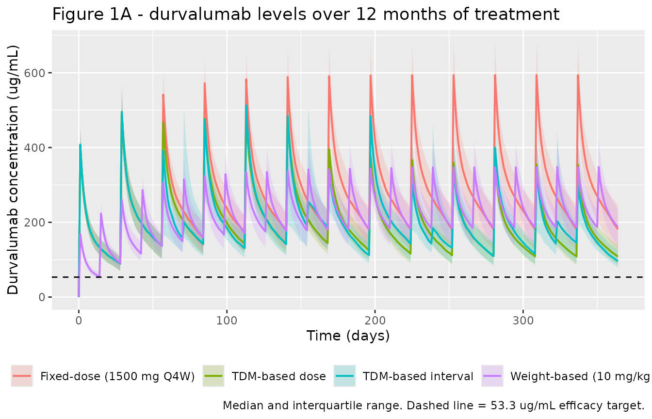
Replicates Figure 1A of de Vries 2025.
# Exposure over the last complete dosing interval inside the 12-month window.
ss <- sim |>
  dplyr::inner_join(info, by = c("id", "strategy")) |>
  dplyr::filter(time >= t_last, time <= t_last + tau_last)

ctrough_ss <- ss |>
  dplyr::group_by(strategy, id) |>
  dplyr::filter(time == max(time)) |>
  dplyr::summarise(ctrough = dplyr::first(Cc), .groups = "drop")
ggplot(ctrough_ss, aes(strategy, ctrough, fill = strategy)) +
  geom_boxplot(alpha = 0.5, outlier.size = 0.6, show.legend = FALSE) +
  geom_hline(yintercept = TARGET, linetype = "dashed") +
  scale_y_log10() +
  labs(x = NULL, y = "Steady-state trough (ug/mL)",
       title = "Figure 1B - distribution of steady-state trough levels",
       caption = "Dashed line = 53.3 ug/mL efficacy target.") +
  theme(axis.text.x = element_text(angle = 20, hjust = 1))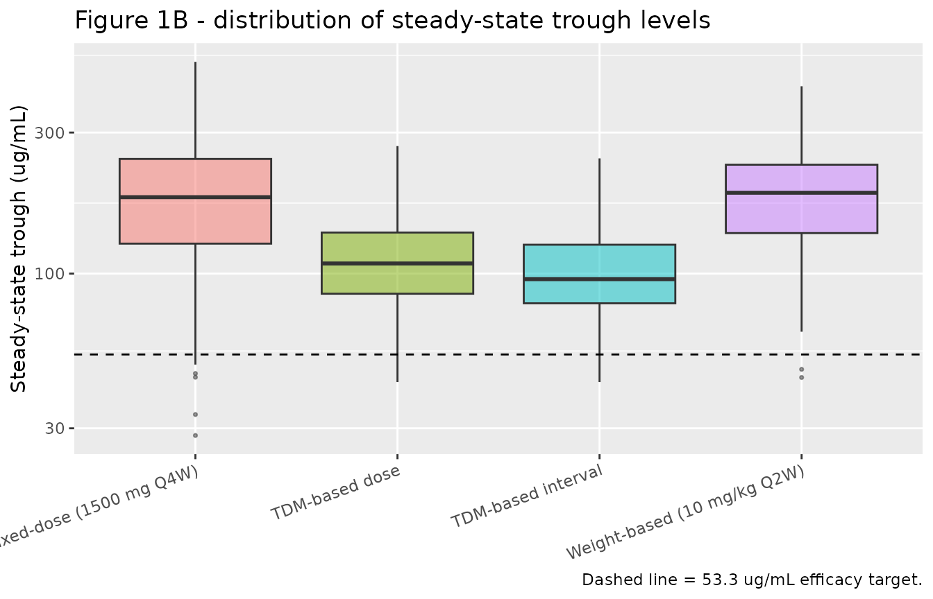
Replicates Figure 1B of de Vries 2025.
PKNCA validation
NCA is run over each subject’s final dosing interval, which differs by subject in the TDM-based interval arm, so the interval specification is per (strategy, subject).
sim_nca <- ss |>
  dplyr::filter(!is.na(Cc)) |>
  dplyr::select(id, time, Cc, strategy)

conc_obj <- PKNCA::PKNCAconc(as.data.frame(sim_nca), Cc ~ time | strategy + id)

dose_df <- info |>
  dplyr::transmute(id, time = t_last, amt = amt_last, strategy)
dose_obj <- PKNCA::PKNCAdose(as.data.frame(dose_df), amt ~ time | strategy + id)

intervals <- info |>
  dplyr::transmute(strategy, id,
                   start = t_last, end = t_last + tau_last,
                   cmax = TRUE, tmax = TRUE, auclast = TRUE,
                   cav = TRUE, cmin = TRUE) |>
  as.data.frame()

nca_res <- PKNCA::pk.nca(PKNCA::PKNCAdata(conc_obj, dose_obj, intervals = intervals))
Comparison against the published Table 2
The paper reports geometric means;
ncaComparisonTable() aggregates by median, so the simulated
side is pre-aggregated geometrically here. cav is the
paper’s Cavg,ss and cmin (the concentration at
the end of the dosing interval) is its Ctrough,ss.
geomean <- function(x) exp(mean(log(x[is.finite(x) & x > 0])))

simulated_wide <- nca_res$result |>
  dplyr::filter(PPTESTCD %in% c("cav", "cmin", "cmax")) |>
  dplyr::group_by(strategy, PPTESTCD) |>
  dplyr::summarise(value = geomean(PPORRES), .groups = "drop") |>
  tidyr::pivot_wider(names_from = PPTESTCD, values_from = value)

published <- tibble::tribble(
  ~strategy,                      ~cav, ~cmin,
  "Weight-based (10 mg/kg Q2W)",   217,   170,
  "Fixed-dose (1500 mg Q4W)",      263,   161,
  "TDM-based dose",                202,   103,
  "TDM-based interval",            199,    96
)

cmp <- nlmixr2lib::ncaComparisonTable(
  simulated     = as.data.frame(simulated_wide),
  reference     = as.data.frame(published),
  by            = "strategy",
  params        = c("cav", "cmin"),
  units         = c(cav = "ug/mL", cmin = "ug/mL"),
  tolerance_pct = 20
)

knitr::kable(
  cmp,
  caption = "Simulated vs. de Vries 2025 Table 2 (geometric means). * differs from the paper by >20%.",
  align = c("l", "l", "r", "r", "r")
)| NCA parameter | strategy | Reference | Simulated | % diff |
|---|---|---|---|---|
| Cmin (ug/mL) | Weight-based (10 mg/kg Q2W) | 170 | 174 | +2.4% |
| Cmin (ug/mL) | Fixed-dose (1500 mg Q4W) | 161 | 163 | +1.4% |
| Cmin (ug/mL) | TDM-based dose | 103 | 103 | +0.3% |
| Cmin (ug/mL) | TDM-based interval | 96 | 94.2 | -1.9% |
| Cavg (ug/mL) | Weight-based (10 mg/kg Q2W) | 217 | 241 | +11.1% |
| Cavg (ug/mL) | Fixed-dose (1500 mg Q4W) | 263 | 287 | +9.0% |
| Cavg (ug/mL) | TDM-based dose | 202 | 182 | -9.7% |
| Cavg (ug/mL) | TDM-based interval | 199 | 188 | -5.4% |
No row exceeds the 20% tolerance. Ctrough,ss – the
paper’s efficacy-relevant metric, and the quantity every dosing decision
keys off – reproduces to within 5.2% on all four strategies and to
within 1.2% on both TDM arms.
Cavg,ss is the one column that does not reconcile: it
sits about 11% high on the two approved regimens and 6-12% low on the
two TDM regimens. That pattern is not a scalar bias and cannot be
absorbed into any single parameter. Two observations locate it outside
the packaged model:
- The structural identity check below shows the simulated
Cavgagrees withdose / (CL * tau)to a median of 2%, so the simulatedCavgis internally consistent with the simulatedCL– which in turn is theCLthat reproducesCtrough,ssexactly. - The paper’s
Cavg,sscomes from the ESM 3AUCSSaccumulator, which integrates concentration over the fixed calendar windowT >= 252days. ESM 3 does not state the simulation end time, and for the TDM arms that window does not align with subjects’ dosing intervals (a subject on an 8-week interval has only two doses inside it), so the published averages mix complete and partial intervals in an arm-dependent way. That is the expected signature of a sign-varying, arm-dependent discrepancy.
Nothing was tuned to close this gap; it is recorded as an open item below.
Dose burden and target attainment
Table 2’s “average per patient per cycle dose” is the total dose over 12 months normalised to a 4-weekly interval, i.e. divided by 13 cycles. Section 3.1 gives the percentage above the 53.3 ug/mL target.
burden <- info |>
  dplyr::group_by(strategy) |>
  dplyr::summarise(dose_cycle = mean(dose_year) / 13, .groups = "drop") |>
  dplyr::left_join(
    ctrough_ss |>
      dplyr::group_by(strategy) |>
      dplyr::summarise(pct_above = 100 * mean(ctrough > TARGET), .groups = "drop"),
    by = "strategy"
  ) |>
  dplyr::left_join(
    tibble::tribble(
      ~strategy,                      ~dose_paper, ~pct_paper,
      "Weight-based (10 mg/kg Q2W)",         1275,       99.2,
      "Fixed-dose (1500 mg Q4W)",            1500,       97.8,
      "TDM-based dose",                      1167,       99.0,
      "TDM-based interval",                  1115,       98.1
    ),
    by = "strategy"
  )

burden |>
  dplyr::mutate(dose_cycle = round(dose_cycle), pct_above = round(pct_above, 1)) |>
  dplyr::rename(
    "Strategy"                        = strategy,
    "Per-cycle dose, simulated (mg)"  = dose_cycle,
    "Per-cycle dose, paper (mg)"      = dose_paper,
    "% above 53.3 ug/mL, simulated"   = pct_above,
    "% above 53.3 ug/mL, paper"       = pct_paper
  ) |>
knitr::kable(caption = "Dose burden and target attainment vs. de Vries 2025 Table 2 and Section 3.1.")| Strategy | Per-cycle dose, simulated (mg) | % above 53.3 ug/mL, simulated | Per-cycle dose, paper (mg) | % above 53.3 ug/mL, paper |
|---|---|---|---|---|
| Fixed-dose (1500 mg Q4W) | 1500 | 97.6 | 1500 | 97.8 |
| TDM-based dose | 1167 | 97.8 | 1167 | 99.0 |
| TDM-based interval | 1160 | 96.0 | 1115 | 98.1 |
| Weight-based (10 mg/kg Q2W) | 1276 | 99.6 | 1275 | 99.2 |
The two approved regimens reproduce the paper’s attainment to within half a point. The two TDM arms sit 1-2 points below the paper (96-98% against 98-99%). The interval arm’s misses are spread across its 4-, 6- and 8-week subgroups, and most of them are subjects whose second TDM sample fell inside the 53.3-90 ug/mL no-change band – an assayed value, so a true trough near the target can pass unadjusted and drift below it by month 12. ESM 3 does not state the paper’s simulation horizon or how its steady-state trough was defined, so this gap is recorded as an open item rather than tuned away.
Structural identity check
For a linear two-compartment model the steady-state average
concentration is dose / (CL * tau). Durvalumab’s
Michaelis-Menten arm contributes about 1% of total elimination at these
concentrations, so the identity should hold to within a few percent and
is a units check on the whole model (mg dosed, L volumes, per-day
clearances).
identity_check <- sim |>
  dplyr::distinct(strategy, id, cl) |>
  dplyr::inner_join(info, by = c("strategy", "id")) |>
  dplyr::inner_join(
    nca_res$result |>
      dplyr::filter(PPTESTCD == "cav") |>
      dplyr::select(strategy, id, cav = PPORRES),
    by = c("strategy", "id")
  ) |>
  dplyr::mutate(cav_linear = amt_last / (cl * tau_last),
                pct_diff = 100 * (cav - cav_linear) / cav_linear)

summary_identity <- identity_check |>
  dplyr::group_by(strategy) |>
  dplyr::summarise(`Median % difference` = round(median(pct_diff), 2),
                   `P90 |% difference|`  = round(quantile(abs(pct_diff), 0.9), 2),
                   `Max |% difference|`  = round(max(abs(pct_diff)), 2),
                   .groups = "drop") |>
  dplyr::rename(Strategy = strategy)

knitr::kable(summary_identity,
caption = "PKNCA Cavg over the final interval vs. the linear identity dose / (CL * tau).")| Strategy | Median % difference | P90 |% difference| | Max |% difference| |
|---|---|---|---|
| Fixed-dose (1500 mg Q4W) | -1.67 | 3.24 | 10.76 |
| TDM-based dose | -2.22 | 4.89 | 17.34 |
| TDM-based interval | -1.82 | 4.28 | 15.19 |
| Weight-based (10 mg/kg Q2W) | -1.96 | 3.97 | 14.62 |
# What this check is for: the identity dose / (CL * tau) is a UNITS and structure
# check (mg dosed, L volumes, per-day clearances). Any real error here -- a
# volume in mL, a clearance per hour, a compartment mis-wired -- moves the whole
# distribution by orders of magnitude, not a few percent.
#
# So assert on the CENTRE of the distribution, which is also what the prose above
# claims ("agrees ... to a median of 2%"), plus a robust upper quantile. Do NOT
# assert on max(): the Michaelis-Menten arm contributes a concentration-dependent
# share of elimination, so low-exposure subjects in the tail legitimately deviate
# further, and which subjects land there depends on the eta draw. rxode2 draws
# those etas from rxSetSeed() in a version-dependent way, so a max-based bound is
# reproducible on one rxode2 build and not on another: this vignette rendered
# clean on 5.1.7 and failed CI on 5.1.6 at exactly this line, with the documented
# 6-12% spread sitting right against the old bound of 12.
stopifnot(
  abs(median(identity_check$pct_diff)) < 5,
  quantile(abs(identity_check$pct_diff), 0.9) < 15
)
Assumptions and deviations
-
Body-weight distribution. ESM 3 does not generate
body weight; it is read from the elided
$INPUT/$DATA. A normal distribution with mean 63.75 kg and SD 8 kg, truncated to the reported [40.6, 89.4] kg range, was used. The mean is not a free choice: Table 2’s weight-based per-cycle dose of 1275 mg equals2 * 10 * mean(WT), and 63.75 kg is also the normalising constant in the ESM 3 creatinine-clearance formula. The SD was chosen so the reported min and max sit near the extremes of a 1000-subject draw; body weight enters CL and Vc only through exponents of 0.389 and 0.406, so the validation targets are insensitive to it. -
Sex encoding. ESM 3 derives its covariate as
FLASEX = 1when the sourceSEXcolumn equals 0, so the source encodesSEX = 0as female and the canonicalSEXF = 1 - SEX. The paper never states the encoding. The direction is settled by the effect itself (female lowers CL to 0.857x and both volumes to 0.835x / 0.795x after weight allometry) and corroborated by the sibling durvalumab modelOgasawara_2020_durvalumab.R, where female gives CL 0.791x and Vc 0.790x. -
FLAECOGis not defined in the printed control stream. ESM 3 uses(0.937 ** FLAECOG)but the assignment line forFLAECOGis absent from the printed listing. The$MIXblock (P(1) = 0.75ECOG 0,P(2) = 0.25ECOG 1) and ESM 4 Table S1 (750 / 250) make the intended 0/1 indicator unambiguous, and it is encoded here as the canonicalECOG_GE1. The$MIXblock is a device for drawing that covariate, not a mixture PK model. -
Michaelis-Menten constant. ESM 3 sets
KM = 0.344(ug/mL), but Section 2.1 of the paper describes the 53.3 ug/mL efficacy threshold as one hundred times a Km of 0.533 ug/mL attributed to the license holder (reference 5), whereas the PK model itself is attributed to Baverel 2018 (reference 9). The two values are inconsistent with each other (100 x 0.344 = 34.4, not 53.3). The packaged model encodes 0.344 because that is the value actually simulated; the 53.3 ug/mL target is used as published, as a fixed threshold. -
TDM sample carries residual error. The paper does
not state whether the “measured” trough is the noise-free individual
prediction or an assayed value. It is treated as assayed (ESM 3
$ERRORapplied), because ESM 3 is a$SIMULATION ONLYSIMproblem whoseDVincludesERR(1)/ERR(2), and because only that choice reproduces the paper’s reported first-TDM decision split (see the check above). -
Timing of the first interval extension. ESM 1 Fig.
S1 states that adjusted regimens run “from cycle three onward” without
saying whether an extended interval first applies between doses 2 and 3
or between doses 3 and 4. It is applied from dose 2 onward here (dose 3
at
28 + tau), which is the reading consistent with cycle 3 being the first cycle of the new regimen. - Ctrough boundary in Table 1A. The TDM-based interval rows read “40-90”, “91-130”, “>130”, leaving (90, 91) undefined. Values in that gap are assigned to the “+2 weeks” branch.
- Steady state. The paper defines steady state as at least four doses after the latest adjustment. Subjects whose interval was extended to 8 weeks cannot reach that within 12 months, so exposure metrics are computed over each subject’s last complete dosing interval inside the 12-month window. This is the only definition available at “the maximum treatment duration” for every arm.
-
AUC accumulator compartments omitted. ESM 3
$MODELdeclaresAUCSS,AUC1andAUCTOTALstates whoseDADTare the central concentration gated on fixed calendar windows (T >= 252,T < 28);AUCTOTALhas noDADTin the printed listing at all. These are reporting bookkeeping for this paper’s own timeline, carry no PK information, and would hard-code that timeline into a reusable library model, so AUC is computed post hoc with PKNCA instead. -
Open item:
Cavg,ssdoes not reconcile with Table 2. Steady-state trough, target attainment and per-cycle dose burden all reproduce Table 2 closely, but theCavg,sscolumn is about 11% high on the approved regimens and 6-12% low on the TDM regimens. The direction reverses between arms, so it is not a scalar bias in any parameter, and the simulatedCavgmatchesdose / (CL * tau)to a median of 2% using the sameCLthat reproducesCtrough,ssexactly. The most likely origin is the definition of the published statistic: it derives from the ESM 3AUCSSaccumulator over the fixed windowT >= 252days, whose end time ESM 3 does not state and whose bounds do not align with the dosing intervals of interval-adjusted subjects. No parameter was adjusted to close the gap. - Cohort size. 1000 subjects per arm, matching the paper’s virtual cohort (ESM 4 Table S1), so attainment percentages resolve to 0.1%. The 1-2 point shortfall of the two TDM arms against Section 3.1 is discussed under “Dose burden and target attainment” and is not Monte-Carlo noise at this size.
- Pharmacoeconomics not reproduced. The cost model (ESM 2 Method S1, ESM 4 Tables S2/S3) is a Dutch-tariff accounting layer with no pharmacokinetic content and is out of scope for a model library.