Abemaciclib (Tate 2018)

Model and source

#> ℹ parameter labels from comments will be replaced by 'label()'
#> Warning: some etas defaulted to non-mu referenced, possible parsing error: etaiov_cl_1, etaiov_cl_2, etaiov_cl_3, etaiov_cl_4
#> as a work-around try putting the mu-referenced expression on a simple line

• Citation: Tate SC, Sykes AK, Kulanthaivel P, Chan EM, Turner PK, Cronier DM. A Population Pharmacokinetic and Pharmacodynamic Analysis of Abemaciclib in a Phase I Clinical Trial in Cancer Patients. Clin Pharmacokinet. 2018;57(3):335-344. doi:10.1007/s40262-017-0559-8.

• Article: https://doi.org/10.1007/s40262-017-0559-8

• Description: One-compartment population PK model with first-order absorption and linear elimination for oral abemaciclib in 224 adults with advanced cancer from the phase I first-in-human study NCT01394016 (Tate 2018). Apparent clearance and volume are fixed per patient; all exposure variability is carried by a relative bioavailability (Frel) that is both dose- and time-dependent. Frel starts at Frel,i = 1 (fixed) at the first dose and decays exponentially (half-life 14.7 days) towards a dose-dependent steady-state value Frel,ss = D50 / (D50 + Dose) with D50 = 101 mg, so repeated dosing at higher doses absorbs proportionally less drug. Serum albumin (power) and alkaline phosphatase (linear deviation) act on the global Frel. Log-normal IIV on Frel,i, Frel,ss, ka and CL/F, inter-occasion variability on CL/F, and combined additive + proportional residual error.

The article is open access (PMC5814509). Its electronic supplement holds three figures only (goodness-of-fit plots, per-dose VPCs and non-retained covariate panels); every parameter is in Table 3 and its two footnotes. No erratum is listed for the article.

The paper’s PK/PD section (Sect. 2.7, Fig. 3) re-uses the previously published mouse-xenograft p-Rb model of Tate 2014 (Clin Cancer Res 20:3763-74) unchanged, driven by this popPK model. Tate 2018 reports no PD parameter values of its own, so this file carries the popPK model only; the p-Rb layer belongs to the Tate 2014 extraction.

Population

The model was fitted to 4012 plasma concentrations from 224 adults with advanced cancer in the phase I study NCT01394016 (Tate 2018 Tables 1 and 2): 67% female, 94% White / 2% Black / 4% Asian, median age 61 years (24-85), median weight 70.4 kg (43.6-175), median serum albumin 39 g/L (24-48) and median alkaline phosphatase 81 IU/L (36-1175). Patients received abemaciclib capsules at 50-225 mg q24h or 75-275 mg q12h; most were treated at 150 or 200 mg q12h. Pharmacokinetic sampling covered cycle 1: a single dose on day -3, then continuous dosing from day 1 to day 28 (Sect. 2.3).

str(ui$population)
#> List of 12
#>  $ species       : chr "human"
#>  $ n_subjects    : int 224
#>  $ n_studies     : int 1
#>  $ n_observations: chr "4012 abemaciclib plasma concentrations (Tate 2018 Table 2)"
#>  $ age_range     : chr "24-85 years (median 61)"
#>  $ weight_range  : chr "43.6-175 kg (median 70.4)"
#>  $ sex_female_pct: num 67
#>  $ race_ethnicity: Named num [1:3] 94 2 4
#>   ..- attr(*, "names")= chr [1:3] "White" "Black" "Asian"
#>  $ disease_state : chr "Adults with advanced cancer: mixed tumours (dose escalation), NSCLC, glioblastoma, breast cancer (including HR+"| __truncated__
#>  $ dose_range    : chr "Oral abemaciclib capsules 50-225 mg q24h or 75-275 mg q12h"
#>  $ regions       : chr "Not reported (multicentre)"
#>  $ notes         : chr "Phase I NCT01394016 (Tate 2018 Sect. 2.1, Tables 1-2). PK model built on cycle-1 data: single dose on day -3, c"| __truncated__

Source trace

Element	Value in the model	Source
One-compartment, first-order absorption, linear CL	d/dt(depot), d/dt(central)	Sect. 3.2
lka	log(0.197 /h)	Table 3, final model
lcl	log(35.9 L/h)	Table 3, final model
lvc	log(1050 L)	Table 3, final model
lfdepot (Frel,i)	fixed(log(1))	Table 3, final model (‘1 (fixed)’)
led50 (D50)	log(101 mg)	Table 3, final model
lfdepot_exp_kdes (lambda)	log(0.00197 /h)	Table 3, final model
Frel,ss = 1 - Dose / (D50 + Dose)	fdepot_exp_inf	Eq. 4; Table 3 footnote a
Frel = Frel,ss - (Frel,ss - Frel,i) exp(-lambda t)	frel_typ	Eq. 5
e_alb_fdepot	-1.32, power on (ALB / 39)	Table 3; footnote b
e_alp_fdepot	0.00197, linear on (ALP - 81)	Table 3; footnote b
Covariates act on the global Frel	fdepot <- frel_typ * ...	Table 3 footnote b; Sect. 2.5
etalfdepot	0.734^2	Table 3, IIV Frel,i 73.4
etalfdepot_exp_inf	1.23^2	Table 3, IIV Frel,ss 123
etalka	0.776^2	Table 3, IIV ka 77.6
etalcl	0.296^2	Table 3, IIV CL/F 29.6
etaiov_cl_1..4	0.521^2	Table 3, IOV CL/F 52.1
addSd	14.8 ng/mL	Table 3, residual additive
propSd	0.171	Table 3, residual proportional 17.1%
Cc = 1000 * central / vc	ng/mL from mg and L	Unit conversion

The equations of Sect. 2.5 and Eqs. 4-5 are rendered as images in the PDF; their text was checked against the <tex-math> of the EuropePMC JATS XML.

The dose- and time-dependent bioavailability

Tate 2018 Sect. 3.2 makes four numeric statements about Eqs. 4-5. The typical-value model reproduces each of them. The origin of t in Eq. 5 is not stated; counting from the day -3 lead-in dose (three days before continuous dosing starts, as drawn in Fig. 1) gives the end of cycle 1 at 720 h.

mod_typ <- rxode2::zeroRe(ui)
#> Warning: some etas defaulted to non-mu referenced, possible parsing error: etaiov_cl_1, etaiov_cl_2, etaiov_cl_3, etaiov_cl_4
#> as a work-around try putting the mu-referenced expression on a simple line

frel_at <- function(dose, t_first) {
  ev <- data.frame(
    id = 1, time = c(0, t_first), amt = c(dose, dose), evid = 1,
    cmt = "depot", ALB = 39, ALP = 81, OCC = 1, T_FIRSTDOSE = c(0, t_first)
  )
  out <- rxode2::rxSolve(mod_typ, ev, addDosing = TRUE, returnType = "data.frame")
  out$fdepot[out$time == t_first & out$evid == 1]
}

claims <- data.frame(t_origin = c("day -3 lead-in dose", "day 1 (continuous start)"),
                     t_end_c1 = c(720, 672))
claims$frel_150 <- sapply(claims$t_end_c1, function(t) frel_at(150, t))
#> ℹ omega/sigma items treated as zero: 'etalfdepot', 'etalfdepot_exp_inf', 'etalka', 'etalcl', 'etaiov_cl_1', 'etaiov_cl_2', 'etaiov_cl_3', 'etaiov_cl_4'
#> ℹ omega/sigma items treated as zero: 'etalfdepot', 'etalfdepot_exp_inf', 'etalka', 'etalcl', 'etaiov_cl_1', 'etaiov_cl_2', 'etaiov_cl_3', 'etaiov_cl_4'
claims$frel_200 <- sapply(claims$t_end_c1, function(t) frel_at(200, t))
#> ℹ omega/sigma items treated as zero: 'etalfdepot', 'etalfdepot_exp_inf', 'etalka', 'etalcl', 'etaiov_cl_1', 'etaiov_cl_2', 'etaiov_cl_3', 'etaiov_cl_4'
#> ℹ omega/sigma items treated as zero: 'etalfdepot', 'etalfdepot_exp_inf', 'etalka', 'etalcl', 'etaiov_cl_1', 'etaiov_cl_2', 'etaiov_cl_3', 'etaiov_cl_4'
claims$pct_more_drug <- 100 * (200 * claims$frel_200 / (150 * claims$frel_150) - 1)

claims |>
  dplyr::mutate(dplyr::across(c(frel_150, frel_200), ~ round(.x, 3)),
                pct_more_drug = round(pct_more_drug, 1)) |>
  dplyr::rename("Origin of t" = t_origin, "End of cycle 1 (h)" = t_end_c1,
                "Frel, 150 mg" = frel_150, "Frel, 200 mg" = frel_200,
                "Extra drug absorbed, 200 vs 150 mg (%)" = pct_more_drug) |>
  knitr::kable()

Origin of t	End of cycle 1 (h)	Frel, 150 mg	Frel, 200 mg	Extra drug absorbed, 200 vs 150 mg (%)
day -3 lead-in dose	720	0.547	0.496	21.0
day 1 (continuous start)	672	0.561	0.512	21.7

lambda <- exp(ui$theta[["lfdepot_exp_kdes"]])
half_life_days <- log(2) / lambda / 24
c(half_life_days = half_life_days, five_half_lives_days = 5 * half_life_days)
#>       half_life_days five_half_lives_days 
#>             14.66047             73.30237

stopifnot(
  # 'approximately 0.55 for a 150 mg dose, and 0.50 for a 200 mg dose'
  abs(claims$frel_150[1] - 0.55) < 0.01,
  abs(claims$frel_200[1] - 0.50) < 0.01,
  # 'for a 33% increase in dose ... increases by only 21%'
  round(claims$pct_more_drug[1]) == 21,
  # 'the half-life for the transition ... is estimated to be 14 days'
  round(half_life_days) %in% c(14, 15)
)

Both origins match the two Frel values; only the day -3 origin gives the quoted 21% (the day 1 origin gives 21.7%, which rounds to 22%), so the model documents T_FIRSTDOSE as time since the very first dose.

Scale of the IIV percentages

Table 3 prints IIV as a bare percentage without saying whether it is omega x 100 (variance = (P/100)^2) or a CV (variance = log(1 + CV^2)). The two readings differ a lot for the wide rows (Frel,ss 123%: 1.51 vs 0.92). Fig. 1b, the VPC for 200 mg q12h from 1000 simulated patients, settles it. Read off the vector figure, the 5th / 50th / 95th percentiles are about 84 / 430 / 1850 ng/mL at plot day 12 (15 days after the first dose) and 69 / 337 / 1570 ng/mL at plot day 25 (28 days).

Below, a large closed-form Monte Carlo (average steady-state concentration, covariates drawn around the cohort medians, residual error included) gives the percentiles under each reading. It is a check on the variance scale, not a cohort simulation, so it uses many draws.

set.seed(2018)
n_mc <- 20000
cv <- c(frel_i = 73.4, frel_ss = 123, cl = 29.6, iov_cl = 52.1)

mc_percentiles <- function(variance, t_days) {
  e <- sapply(variance, function(v) rnorm(n_mc, 0, sqrt(v)))
  alb <- pmin(pmax(39 * exp(rnorm(n_mc, 0, 0.11)), 24), 48)
  alp <- pmin(pmax(81 * exp(rnorm(n_mc, 0, sqrt(log(1 + 1.03^2)))), 36), 1175)
  fss <- 101 / (101 + 200) * exp(e[, "frel_ss"])
  fi <- exp(e[, "frel_i"])
  frel <- (fss - (fss - fi) * exp(-0.00197 * t_days * 24)) *
    (alb / 39)^-1.32 * (1 + 0.00197 * (alp - 81))
  cavg <- 1000 * frel * 200 / 12 / (35.9 * exp(e[, "cl"] + e[, "iov_cl"]))
  y <- cavg * (1 + rnorm(n_mc, 0, 0.171)) + rnorm(n_mc, 0, 14.8)
  stats::quantile(y, c(0.05, 0.5, 0.95), names = FALSE)
}

scale_check <- tidyr::expand_grid(
  reading = c("omega x 100", "CV, log(1 + CV^2)"),
  t_days = c(15, 28)
)
scale_check <- scale_check |>
  dplyr::rowwise() |>
  dplyr::mutate(q = list(mc_percentiles(
    if (reading == "omega x 100") (cv / 100)^2 else log(1 + (cv / 100)^2),
    t_days
  ))) |>
  dplyr::ungroup() |>
  dplyr::mutate(p05 = sapply(q, `[`, 1), p50 = sapply(q, `[`, 2), p95 = sapply(q, `[`, 3)) |>
  dplyr::select(-q)

fig1b <- data.frame(t_days = c(15, 28), fig_p05 = c(84, 69), fig_p50 = c(430, 337),
                    fig_p95 = c(1850, 1570))
scale_check <- dplyr::left_join(scale_check, fig1b, by = "t_days") |>
  dplyr::mutate(p95_diff_pct = 100 * (p95 / fig_p95 - 1))

scale_check |>
  dplyr::mutate(dplyr::across(c(p05, p50, p95), ~ round(.x)),
                p95_diff_pct = round(p95_diff_pct)) |>
  dplyr::rename("Reading" = reading, "Days since first dose" = t_days,
                "Sim P5" = p05, "Sim P50" = p50, "Sim P95" = p95,
                "Fig. 1b P5" = fig_p05, "Fig. 1b P50" = fig_p50, "Fig. 1b P95" = fig_p95,
                "P95 vs figure (%)" = p95_diff_pct) |>
  knitr::kable()

Reading	Days since first dose	Sim P5	Sim P50	Sim P95	Fig. 1b P5	Fig. 1b P50	Fig. 1b P95	P95 vs figure (%)
omega x 100	15	81	383	1887	84	430	1850	2
omega x 100	28	60	300	1601	69	337	1570	2
CV, log(1 + CV^2)	15	87	361	1462	84	430	1850	-21
CV, log(1 + CV^2)	28	67	282	1230	69	337	1570	-22

stopifnot(
  # The omega x 100 reading reproduces the upper edge of the published band
  # within digitisation error; the log(1 + CV^2) reading is about 20% narrow.
  all(abs(scale_check$p95_diff_pct[scale_check$reading == "omega x 100"]) < 12),
  all(scale_check$p95_diff_pct[scale_check$reading != "omega x 100"] < -15)
)

The omega x 100 reading matches the band; the model therefore uses variance = (P/100)^2 for every IIV and IOV term.

Virtual cohort and VPC

Two arms, 150 and 200 mg q12h, with the NCT01394016 cycle-1 design: a single dose at time 0 (day -3), continuous q12h dosing from 72 h (day 1), and a final morning dose on day 28 (720 h) with no evening dose, followed by 24 h of sampling. Serum albumin and alkaline phosphatase are drawn per subject around the Table 1 medians and clipped to the observed ranges. Occasions follow the four PK sampling visits (day -3, 15, 22 and 28).

n_per_arm <- 200
dose_times <- c(0, seq(72, 720, by = 12))
obs_times <- sort(unique(c(seq(0, 744, by = 2), 0:24, 720:744)))

make_arm <- function(dose_mg, id_offset) {
  ids <- id_offset + seq_len(n_per_arm)
  cov <- data.frame(
    id = ids,
    ALB = pmin(pmax(39 * exp(rnorm(n_per_arm, 0, 0.11)), 24), 48),
    ALP = pmin(pmax(81 * exp(rnorm(n_per_arm, 0, sqrt(log(1 + 1.03^2)))), 36), 1175)
  )
  doses <- tidyr::expand_grid(id = ids, time = dose_times) |>
    dplyr::mutate(amt = dose_mg, evid = 1, cmt = "depot")
  obs <- tidyr::expand_grid(id = ids, time = obs_times) |>
    dplyr::mutate(amt = 0, evid = 0, cmt = "central")
  dplyr::bind_rows(doses, obs) |>
    dplyr::left_join(cov, by = "id") |>
    dplyr::mutate(
      treatment = paste0(dose_mg, " mg q12h"),
      T_FIRSTDOSE = time,
      OCC = dplyr::case_when(time < 72 ~ 1, time < 408 ~ 2, time < 576 ~ 3, TRUE ~ 4)
    ) |>
    dplyr::arrange(id, time, dplyr::desc(evid))
}

set.seed(5814509)
events <- dplyr::bind_rows(make_arm(150, 0), make_arm(200, 1000))

rxode2::rxSetSeed(5814509)
sim <- rxode2::rxSolve(ui, events, keep = c("treatment"), returnType = "data.frame")

# The pre-dose time-zero row is all zeros and cannot be drawn on a log axis.
vpc <- sim |>
  dplyr::mutate(day = time / 24 - 3) |>
  dplyr::filter(day > -3) |>
  dplyr::group_by(treatment, time, day) |>
  dplyr::summarise(
    p05 = stats::quantile(sim, 0.05), p50 = stats::median(sim), p95 = stats::quantile(sim, 0.95),
    .groups = "drop"
  )

ggplot(vpc, aes(day)) +
  geom_line(aes(y = p50)) +
  geom_line(aes(y = p05), linetype = "dotted") +
  geom_line(aes(y = p95), linetype = "dotted") +
  facet_wrap(~treatment, ncol = 1) +
  scale_y_log10(limits = c(1, 3000)) +
  labs(x = "Time (days)", y = "Abemaciclib plasma concentration (ng/mL)") +
  theme_bw()
#> Warning in transformation$transform(x): NaNs produced
#> Warning in scale_y_log10(limits = c(1, 3000)): log-10 transformation introduced
#> infinite values.
#> Warning: Removed 4 rows containing missing values or values outside the scale range
#> (`geom_line()`).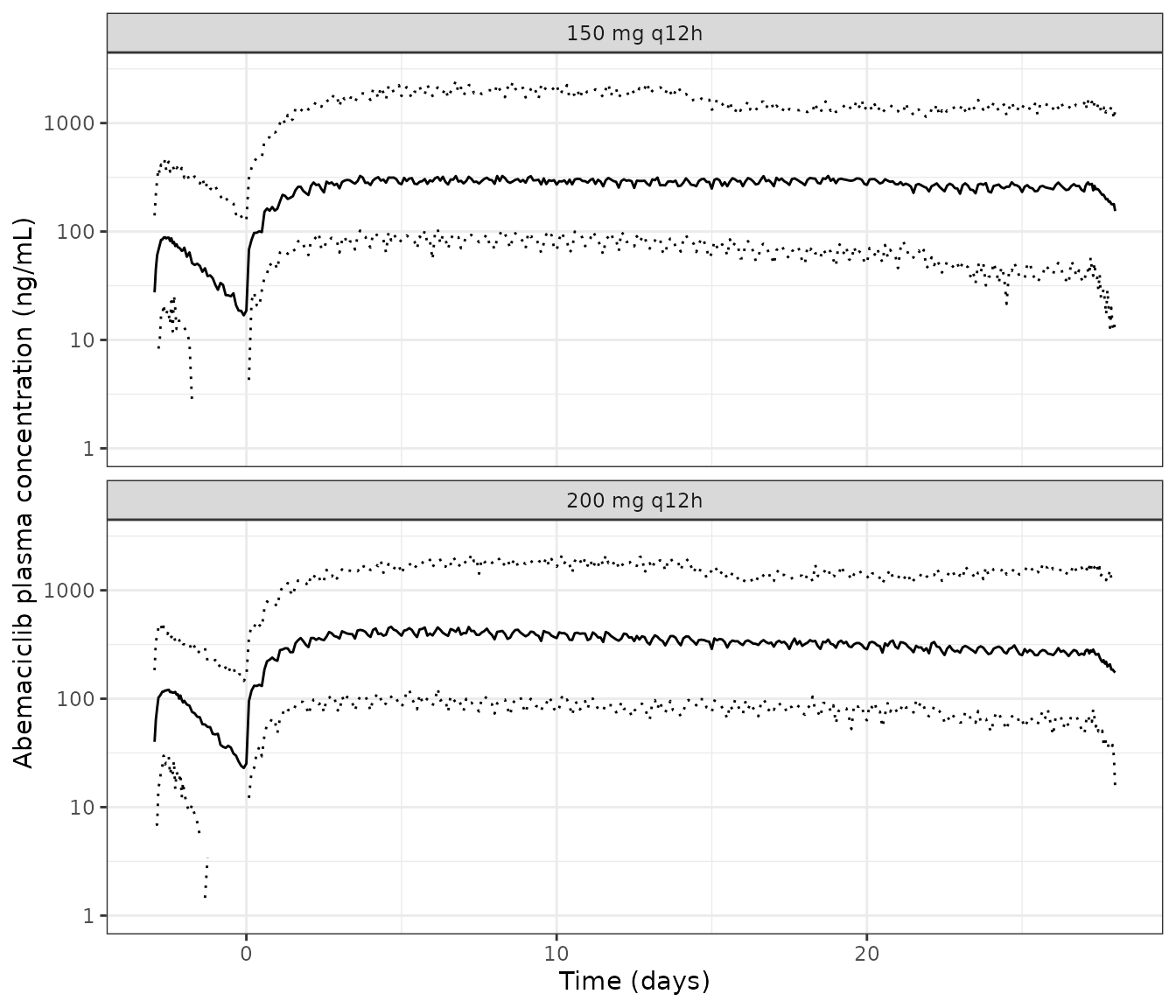

Replicates Figure 1 of Tate 2018: median and 5th/95th percentiles of simulated abemaciclib concentrations after 150 mg (top) and 200 mg (bottom) q12h. Plot day 0 is the start of continuous dosing; the lead-in dose is at day -3.

The steady-state band sits at the level and width of Fig. 1: for 200 mg q12h the published median is about 430 ng/mL at plot day 12 and about 340 ng/mL at plot day 25, and the 95th percentile about 1850 and 1570 ng/mL.

vpc_check <- vpc |>
  # Mid-interval (6 h post-dose) rather than at a dose time, so the
  # comparison is not made at the trough of the dosing interval.
  dplyr::filter(treatment == "200 mg q12h", time %in% c(366, 678)) |>
  dplyr::mutate(fig_p50 = ifelse(time == 366, 430, 337))
vpc_check |>
  dplyr::select(time, p05, p50, p95, fig_p50) |>
  dplyr::mutate(dplyr::across(c(p05, p50, p95), ~ round(.x))) |>
  dplyr::rename("Time since first dose (h)" = time, "Sim P5" = p05, "Sim P50" = p50,
                "Sim P95" = p95, "Fig. 1b P50 (digitised)" = fig_p50) |>
  knitr::kable()

Time since first dose (h)	Sim P5	Sim P50	Sim P95	Fig. 1b P50 (digitised)
366	81	394	1773	430
678	68	282	1645	337

stopifnot(
  # Centre of the band within a factor of 1.6 of the digitised median
  # (200 subjects; a single time point; digitisation of a log axis).
  all(vpc_check$p50 / vpc_check$fig_p50 > 1 / 1.6),
  all(vpc_check$p50 / vpc_check$fig_p50 < 1.6)
)

NCA with PKNCA

Tate 2018 does not tabulate NCA results (they are in the phase I clinical report, its reference 8, which was not available when the model was built), so the simulated NCA below is reported for the two arms without a published comparator. Two intervals are summarised: the day -3 single dose (0-72 h) and the day 28 dose (720-744 h).

conc <- sim |>
  dplyr::filter(!is.na(Cc)) |>
  dplyr::select(id, time, Cc, treatment) |>
  as.data.frame()

dose_df <- events |>
  dplyr::filter(evid == 1) |>
  dplyr::select(id, time, amt, treatment) |>
  as.data.frame()

conc_obj <- PKNCA::PKNCAconc(conc, Cc ~ time | treatment + id)
dose_obj <- PKNCA::PKNCAdose(dose_df, amt ~ time | treatment + id)
intervals <- data.frame(
  start = c(0, 720), end = c(72, 744),
  cmax = TRUE, tmax = TRUE, auclast = TRUE, half.life = c(TRUE, FALSE)
)
nca_res <- PKNCA::pk.nca(PKNCA::PKNCAdata(conc_obj, dose_obj, intervals = intervals))
nca_summary <- summary(nca_res)
knitr::kable(nca_summary)

start	end	treatment	N	auclast	cmax	tmax	half.life
0	72	150 mg q12h	200	3710 [110]	101 [100]	11.0 [2.00, 36.0]	24.7 [15.8]
720	744	150 mg q12h	200	5350 [157]	271 [138]	5.00 [2.00, 8.00]	.
0	72	200 mg q12h	200	4800 [109]	131 [97.4]	10.0 [2.00, 50.0]	26.1 [18.7]
720	744	200 mg q12h	200	5940 [127]	297 [117]	4.00 [2.00, 8.00]	.

nca_tbl <- as.data.frame(nca_res$result)
single_dose_cmax <- nca_tbl |>
  dplyr::filter(PPTESTCD == "cmax", start == 0) |>
  dplyr::group_by(treatment) |>
  dplyr::summarise(med = stats::median(PPORRES), .groups = "drop")
day28_cmax <- nca_tbl |>
  dplyr::filter(PPTESTCD == "cmax", start == 720) |>
  dplyr::group_by(treatment) |>
  dplyr::summarise(med = stats::median(PPORRES), .groups = "drop")

# Typical single-dose Cmax from the closed-form one-compartment oral solution,
# Frel = 1 at the first dose.
ka <- 0.197
kel <- 35.9 / 1050
tmax_typ <- log(ka / kel) / (ka - kel)
cmax_typ <- function(dose) 1000 * dose / 1050 * ka / (ka - kel) * (exp(-kel * tmax_typ) - exp(-ka * tmax_typ))
c(tmax_typ_h = tmax_typ, cmax_150 = cmax_typ(150), cmax_200 = cmax_typ(200))
#> tmax_typ_h   cmax_150   cmax_200 
#>   10.75648   98.89672  131.86230

stopifnot(
  # Medians of the single-dose Cmax sit near the typical value: Frel,i, ka
  # and CL vary log-symmetrically around it.
  abs(single_dose_cmax$med[single_dose_cmax$treatment == "200 mg q12h"] / cmax_typ(200) - 1) < 0.25,
  # Day 28 exposure is higher than single dose (accumulation outweighs the
  # fall in Frel at both doses).
  all(day28_cmax$med > single_dose_cmax$med)
)

Terminal half-life of the typical patient is ln(2) x Vd/F / (CL/F) = 20.3 h.

Assumptions and deviations

• IIV scale. Table 3 does not state whether its IIV percentages are omega x 100 or CVs; the model uses variance = (P/100)^2 because that reading reproduces the Fig. 1b VPC band (section above). This also governs the IOV on CL/F.
• Origin of t in Eq. 5. Not stated in the paper. T_FIRSTDOSE counts from the very first dose (the day -3 lead-in), which reproduces the Sect. 3.2 statements exactly; counting from day 1 would raise Frel by about 0.015 at the end of cycle 1.
• Dose in Eq. 4. Read as the amount of the individual administration (150 or 200 mg), not the daily dose: this reproduces the paper’s Frel values for 150 and 200 mg q12h. It is taken from the event record with podo(depot), so a dose reduction changes Frel,ss from that dose on, and a q24h and a q12h regimen at the same per-dose amount share Frel,ss.
• IIV placement. Section 2.4 states that variability was log-normal. The IIV of Frel,i multiplies Frel,i and the IIV of Frel,ss multiplies the Eq. 4 value, each before Eq. 5 combines them. Covariates multiply the combined Frel (Table 3 footnote b, Sect. 2.5).
• Occasions. The IOV on CL/F is reported without an occasion definition. Four occasions, one per cycle-1 PK sampling visit, are an extraction-side choice; a user with a different occasion structure should set OCC accordingly (records with OCC outside 1-4 carry no IOV).
• Residual error. Additive and proportional components are combined as independent variances (add() + prop()), the NONMEM Y = F + F * EPS(1) + EPS(2) form.
• Naming. Frel,ss is fdepot_exp_inf and lambda is lfdepot_exp_kdes, the registered time-varying _exp_ family transposed to bioavailability (maintainers’ ruling, 2026-09-21). Frel,ss has no typical value of its own, so only its eta (etalfdepot_exp_inf) appears in ini().
• PK/PD. The Fig. 3 p-Rb simulation re-uses the Tate 2014 preclinical model unchanged and is not part of this file.
• Virtual covariates. Albumin and ALP are drawn as log-normal around the Table 1 medians with the Table 1 CVs and held constant within subject; the study updated them at each visit.