Unbound efavirenz, atazanavir and ritonavir (Dumond 2017)
Source:vignettes/articles/Dumond_2017_unbound_antiretrovirals.Rmd
Dumond_2017_unbound_antiretrovirals.RmdModel and source
Dumond 2017 fits three separate population PK models, one per drug, each describing the total and the unbound (protein-free) plasma concentration simultaneously. The three models are therefore packaged as three model files that share this vignette.
mod_names <- c(
  efavirenz = "Dumond_2017_efavirenz",
  atazanavir = "Dumond_2017_atazanavir",
  ritonavir = "Dumond_2017_ritonavir"
)
uis <- lapply(mod_names, function(n) rxode2::rxode(readModelDb(n)))
#> ℹ parameter labels from comments will be replaced by 'label()'
#> Warning: some etas defaulted to non-mu referenced, possible parsing error: etaiov_cl_1, etaiov_cl_2
#> as a work-around try putting the mu-referenced expression on a simple line
#> ℹ parameter labels from comments will be replaced by 'label()'
#> Warning: some etas defaulted to non-mu referenced, possible parsing error: etaiov_cl_1, etaiov_cl_2
#> as a work-around try putting the mu-referenced expression on a simple line
#> ℹ parameter labels from comments will be replaced by 'label()'
#> Warning: some etas defaulted to non-mu referenced, possible parsing error: etaiov_cl_1, etaiov_cl_2
#> as a work-around try putting the mu-referenced expression on a simple line- Citation: Dumond JB, Chen J, Cottrell M, Trezza CR, Prince HMA, Sykes C, Torrice C, White N, Malone S, Wang R, Patterson KB, Sharpless NE, Forrest A. Population pharmacokinetics modeling of unbound efavirenz, atazanavir, and ritonavir in HIV-infected subjects with aging biomarkers. CPT Pharmacometrics Syst Pharmacol. 2017;6(2):128-135. doi:10.1002/psp4.12151.
- Article: https://doi.org/10.1002/psp4.12151
- Supplementary NONMEM control streams (final models, one per drug):
PSP4-6-128-s001.txt(efavirenz),PSP4-6-128-s002.txt(atazanavir),PSP4-6-128-s003.txt(ritonavir), available from the Europe PMC supplementary files for PMC5321807.
| Model | Structure | Covariates |
|---|---|---|
| Dumond_2017_efavirenz | 2 compartments, first-order absorption, no lag | none |
| Dumond_2017_atazanavir | 2 compartments, first-order absorption with lag | none |
| Dumond_2017_ritonavir | 1 compartment, first-order absorption with lag | body weight on CLu/F and Vu/F; BMI < 30 on fu |
Population
Sixty HIV-infected adults taking efavirenz 600 mg once daily and 31 taking atazanavir 300 mg / ritonavir 100 mg once daily were recruited from two North Carolina infectious-disease clinics (ClinicalTrials.gov NCT01180075). Everyone also received tenofovir disoproxil fumarate 300 mg and emtricitabine 200 mg once daily. Median age was 48 years (range 22-73) in the efavirenz arm and 49 years (range 24-61) in the atazanavir/ritonavir arm; 30% and 39% were women and 57% and 61% were African American respectively (Table 1). Median BMI was 27.2 kg/m^2 (range 17.3-44.3) and 30.3 kg/m^2 (range 20.2-40.4).
The study was designed around markers of biologic rather than chronologic aging: every participant was phenotyped with the five-component Fried frailty instrument (2 frail and 8 prefrail in the efavirenz arm; 1 frail and 9 prefrail in the atazanavir/ritonavir arm) and, for the sparsely sampled participants, p16INK4a expression in CD3+ T cells was measured. Most participants gave four samples per occasion over one to three occasions; six per arm gave 11 samples around a single observed dose. Total and unbound concentrations were measured at every sampling time, the unbound concentration by rapid equilibrium dialysis with LC-MS/MS.
The same information is available programmatically via each model’s
population metadata:
str(uis$ritonavir$population, max.level = 1)
#> List of 14
#>  $ species       : chr "human"
#>  $ n_subjects    : int 31
#>  $ n_studies     : int 1
#>  $ age_range     : chr "24-61 years"
#>  $ age_median    : chr "49 years"
#>  $ sex_female_pct: num 39
#>  $ race_ethnicity: Named num [1:3] 61 32 6
#>   ..- attr(*, "names")= chr [1:3] "African American" "White" "Other"
#>  $ disease_state : chr "HIV-1 infection on stable antiretroviral therapy for at least 2 weeks; adherence at least 27 of the previous 30"| __truncated__
#>  $ dose_range    : chr "Ritonavir 100 mg with atazanavir 300 mg by mouth once daily at steady state, co-administered with tenofovir dis"| __truncated__
#>  $ regions       : chr "United States (UNC HealthCare Infectious Diseases Clinic, Chapel Hill NC; Cone Health Regional Center for Infec"| __truncated__
#>  $ bmi_range     : chr "20.2-40.4 kg/m^2 (median 30.3)"
#>  $ renal_function: chr "Creatinine clearance (Cockcroft-Gault) median 100 mL/min (range 67-227)"
#>  $ aging_markers : chr "Fried frailty phenotype: 21 participants (68%) with no positive components, 9 (29%) prefrail with 1-2 component"| __truncated__
#>  $ notes         : chr "Table 1 (ATV/RTV arm, n = 31). 25 participants were sparsely sampled (4 samples per occasion: predose, 2 h, 4-6"| __truncated__
Model structure: the unbound compartment is the central compartment
The paper’s distinguishing feature is that the ODE system is written on the unbound side. The supplementary control streams make this explicit:
$DES
DADT(1) = -KA*A(1)
DADT(2) =  KA*A(1) - CL/V*A(2) - Q/V*A(2) + Q/VP*A(3)
DADT(3) =  Q/V*A(2) - Q/VP*A(3)

$ERROR
CU     = A(2)/V
CTOTAL = CU/FU
so CL, V, Q and
VP are the apparent unbound parameters CLu/F,
Vu/F, Qu/F and Vp,u/F, and the total concentration is recovered by
dividing the unbound concentration by the fraction unbound. The model
files keep the canonical nlmixr2lib names cl,
vc, q, vp for these quantities
(the same convention FernandezRubio_2025_ceftriaxone uses
for a model fitted to free concentrations) and expose both observables,
Cu and Cc.
Table 2 also prints the corresponding total-drug parameters as the products with fu (footnotes a-d). Those products are a free arithmetic check on the transcription, so they are asserted here rather than merely quoted.
theta <- function(ui, nm) {
  if (!nm %in% names(ui$theta)) return(NA_real_)
  unname(ui$theta[[nm]])
}
tab2 <- tibble::tribble(
  ~drug, ~model, ~cl_pub, ~vc_pub, ~q_pub, ~vp_pub,
  # Table 2, rows CL/F, V/F, Q/F and Vp/F (footnotes a-d)
  "Efavirenz", "efavirenz", 6.93, 130, 38.8, 159,
  "Atazanavir", "atazanavir", 5.73, 62.9, 7.61, 129,
  "Ritonavir", "ritonavir", 4.85, 52.9, NA, NA
) |>
  rowwise() |>
  mutate(
    fu = exp(theta(uis[[model]], "lfu")),
    cl_der = exp(theta(uis[[model]], "lcl")) * fu,
    vc_der = exp(theta(uis[[model]], "lvc")) * fu,
    q_der = exp(theta(uis[[model]], "lq")) * fu,
    vp_der = exp(theta(uis[[model]], "lvp")) * fu
  ) |>
  ungroup()

# Every quantity involved is printed to three significant figures, so the
# product of two printed values cannot match a third printed value exactly:
# the rounding of CLu/F alone is worth up to 0.4% on a value like 134. The
# realised deviations across the ten comparisons are 0.03% to 0.21%, so 1% is
# the tolerance. A transcription error anywhere in this chain moves the
# product by at least one printed digit, which is far more than 1%.
rel_dev <- with(tab2, c(
  abs(cl_der / cl_pub - 1), abs(vc_der / vc_pub - 1),
  abs(q_der / q_pub - 1), abs(vp_der / vp_pub - 1)
))
stopifnot(
  # Ritonavir is one-compartment, so exactly two of the twelve cells are NA by
  # design; checking the count keeps the na.rm below from passing vacuously.
  sum(is.na(rel_dev)) == 2L,
  max(rel_dev, na.rm = TRUE) < 0.01
)

tab2 |>
  transmute(
    Drug = drug,
    `fu` = signif(fu, 3),
    `CL/F published (L/h)` = cl_pub, `CL/F = CLu/F x fu` = signif(cl_der, 3),
    `V/F published (L)` = vc_pub, `V/F = Vu/F x fu` = signif(vc_der, 3),
    `Q/F published (L/h)` = q_pub, `Q/F = Qu/F x fu` = signif(q_der, 3),
    `Vp/F published (L)` = vp_pub, `Vp/F = Vp,u/F x fu` = signif(vp_der, 3)
  ) |>
knitr::kable(caption = "Table 2 footnotes a-d: the printed total-drug parameters are reproduced exactly by the packaged unbound parameters times fu.")| Drug | fu | CL/F published (L/h) | CL/F = CLu/F x fu | V/F published (L) | V/F = Vu/F x fu | Q/F published (L/h) | Q/F = Qu/F x fu | Vp/F published (L) | Vp/F = Vp,u/F x fu |
|---|---|---|---|---|---|---|---|---|---|
| Efavirenz | 0.00654 | 6.93 | 6.93 | 130.0 | 130.0 | 38.80 | 38.8 | 159 | 159 |
| Atazanavir | 0.05670 | 5.73 | 5.73 | 62.9 | 62.9 | 7.61 | 7.6 | 129 | 129 |
| Ritonavir | 0.00628 | 4.85 | 4.85 | 52.9 | 52.9 | NA | NA | NA | NA |
Source trace
Per-parameter provenance is recorded as an in-file comment next to
each ini() entry in
inst/modeldb/specificDrugs/Dumond_2017_<drug>.R. The
table below collects the structural entries; the IIV, between-occasion
and residual-error entries all come from the corresponding blocks of the
same table.
| Equation / parameter | EFV | ATV | RTV | Source location |
|---|---|---|---|---|
lcl (CLu/F, L/h) |
1,060 | 101 | 772 (70 kg) | Table 2, row CLu/F
|
lvc (Vu/F, L) |
19,900 | 1,110 | 8,430 (70 kg) | Table 2, row Vu/F
|
lq (Qu/F, L/h) |
5,940 | 134 | n/a | Table 2, row Qu/F
|
lvp (Vp,u/F, L) |
24,300 | 2,280 | n/a | Table 2, row Vp,u/F
|
lka (1/h) |
0.463 | 0.705 | 1.59 | Table 2, row ka
|
ltlag (h) |
n/a | 0.529 | 0.604 | Table 2, row Lag time
|
lfu (fraction) |
0.00654 | 0.0567 | 0.00628 | Table 2, row fu (%)
|
e_wt_cl, e_wt_vc
|
n/a | n/a | 0.75, 1 (fixed) | Methods, “Population pharmacokinetic modeling”; control stream
MU_1 = THETA(1) + 0.75*LWT
|
e_bmi_fu |
n/a | n/a | log(1.52) | Table 2, row Influence of BMI < 30 on fu; footnote
e |
IIV etal* (CV%) |
Table 2 | Table 2 | Table 2 | Table 2, first IIV (CV%) block |
IOV etaiov_cl_* (CV%) |
42.4 | 73.9 | 60.5 | Table 2, second block (headed IIV (CV%); see
Assumptions) |
propSd / propSd_Cu
|
0.242 / 0.313 | 0.276 / 0.301 | 0.414 / 0.344 | Table 2, Residual error (CV%)
|
ODE system, Cu = central/vc,
Cc = Cu/fu
|
n/a | n/a | n/a | Figure 1 schematic; supplementary control streams $DES
and $ERROR
|
Typical-value steady-state profiles
The paper reports no non-compartmental analysis, so the quantitative
anchor is Table 2 itself: at steady state the apparent oral clearance is
Dose / AUC0-tau, separately for the total and the unbound
stream. That recovery is not circular - AUC0-tau comes from
the numerical solve, so it goes red on a mis-wired ODE, a mis-applied
fu, a wrong dose or a wrong absorption route.
tau <- 24
n_doses <- 20L
last_dose <- tau * (n_doses - 1L)
doses <- c(efavirenz = 600, atazanavir = 300, ritonavir = 100)

# Observation grid: dense through absorption, coarser through the tail.
obs_grid <- c(seq(0, 4, by = 0.05), seq(4.1, tau, by = 0.1))

# Event table built as a plain data.frame, with cmt set to the ODE state and an
# explicit dvid on every observation row: these models declare two endpoints, so
# an observation row must say which endpoint it belongs to. Naming the algebraic
# observable in cmt instead would inject a compartment slot and renumber the
# states, so the ODE state name is used.
make_events <- function(ids, dose, t_offsets, covs = NULL) {
  subj <- tibble::tibble(id = ids)
  if (!is.null(covs)) subj <- dplyr::bind_cols(subj, covs)
  subj$OCC <- 1
  dosing <- subj |>
    dplyr::mutate(
      time = 0, amt = dose, evid = 1L, cmt = "depot",
      ii = tau, addl = n_doses - 1L, dvid = NA_integer_
    )
  obs <- tidyr::crossing(subj, tibble::tibble(toff = t_offsets)) |>
    dplyr::mutate(
      time = last_dose + toff, amt = NA_real_, evid = 0L, cmt = "central",
      ii = NA_real_, addl = NA_integer_, dvid = 1L
    )
  dplyr::bind_rows(dosing, obs) |>
    dplyr::arrange(id, time, dplyr::desc(evid)) |>
    as.data.frame()
}

# A typical 70 kg participant with BMI >= 30 (the ritonavir fu reference group),
# so the solve is directly comparable with the starred Table 2 estimates.
solve_typical <- function(drug, t_offsets = obs_grid, WT = 70, BMI = 35) {
  ev <- make_events(1L, doses[[drug]], t_offsets, tibble::tibble(WT = WT, BMI = BMI))
  s <- rxode2::rxSolve(rxode2::zeroRe(uis[[drug]]), ev, omega = NA, returnType = "data.frame")
  # rxSolve omits the id column for a single-subject event table.
  if (is.null(s$id)) s$id <- 1L
  dplyr::mutate(s, drug = drug, toff = time - last_dose)
}
typ <- dplyr::bind_rows(lapply(names(doses), solve_typical))
#> Warning: some etas defaulted to non-mu referenced, possible parsing error: etaiov_cl_1, etaiov_cl_2
#> as a work-around try putting the mu-referenced expression on a simple line
#> Warning: some etas defaulted to non-mu referenced, possible parsing error: etaiov_cl_1, etaiov_cl_2
#> as a work-around try putting the mu-referenced expression on a simple line
#> Warning: some etas defaulted to non-mu referenced, possible parsing error: etaiov_cl_1, etaiov_cl_2
#> as a work-around try putting the mu-referenced expression on a simple line
stopifnot(!anyNA(typ$Cc), !anyNA(typ$Cu), all(typ$Cc > 0), all(typ$Cu > 0))
Steady state must actually have been reached before
Dose / AUC0-tau means anything. The check below re-solves
over the previous dosing interval and compares the two AUCs; it
is deterministic (no cohort, no RNG).
ss_ratio <- vapply(names(doses), function(drug) {
  prev <- solve_typical(drug, t_offsets = obs_grid - tau)
  cur <- dplyr::filter(typ, drug == !!drug)
  a_prev <- PKNCA::pk.calc.auc.last(conc = prev$Cc, time = prev$toff + tau)
  a_cur <- PKNCA::pk.calc.auc.last(conc = cur$Cc, time = cur$toff)
  a_cur / a_prev
}, numeric(1))
#> Warning: some etas defaulted to non-mu referenced, possible parsing error: etaiov_cl_1, etaiov_cl_2
#> as a work-around try putting the mu-referenced expression on a simple line
#> Warning: some etas defaulted to non-mu referenced, possible parsing error: etaiov_cl_1, etaiov_cl_2
#> as a work-around try putting the mu-referenced expression on a simple line
#> Warning: some etas defaulted to non-mu referenced, possible parsing error: etaiov_cl_1, etaiov_cl_2
#> as a work-around try putting the mu-referenced expression on a simple line
# Deterministic quantity: the realised values are within 1e-3 of 1 for all
# three drugs, so a 1% band is loose enough to survive a solver-tolerance
# change and tight enough to fail if 20 doses were not enough.
stopifnot(all(abs(ss_ratio - 1) < 0.01))
round(ss_ratio, 5)
#>  efavirenz atazanavir  ritonavir
#>    1.00001    1.00002    1.00000
typ |>
  dplyr::select(drug, toff, Total = Cc, Unbound = Cu) |>
  tidyr::pivot_longer(c(Total, Unbound), names_to = "analyte", values_to = "conc") |>
  dplyr::mutate(
    conc_ngml = conc * 1000,
    drug = factor(drug, levels = names(doses), labels = c("Efavirenz", "Atazanavir", "Ritonavir"))
  ) |>
  ggplot(aes(toff, conc_ngml)) +
  geom_line(linewidth = 0.8) +
  facet_grid(drug ~ analyte, scales = "free_y") +
  scale_y_log10() +
  labs(
    x = "Time after last dose (h)", y = "Concentration (ng/mL)",
    caption = "Compare with Figure 2a-c of Dumond 2017 (prediction medians)."
  ) +
  theme_bw()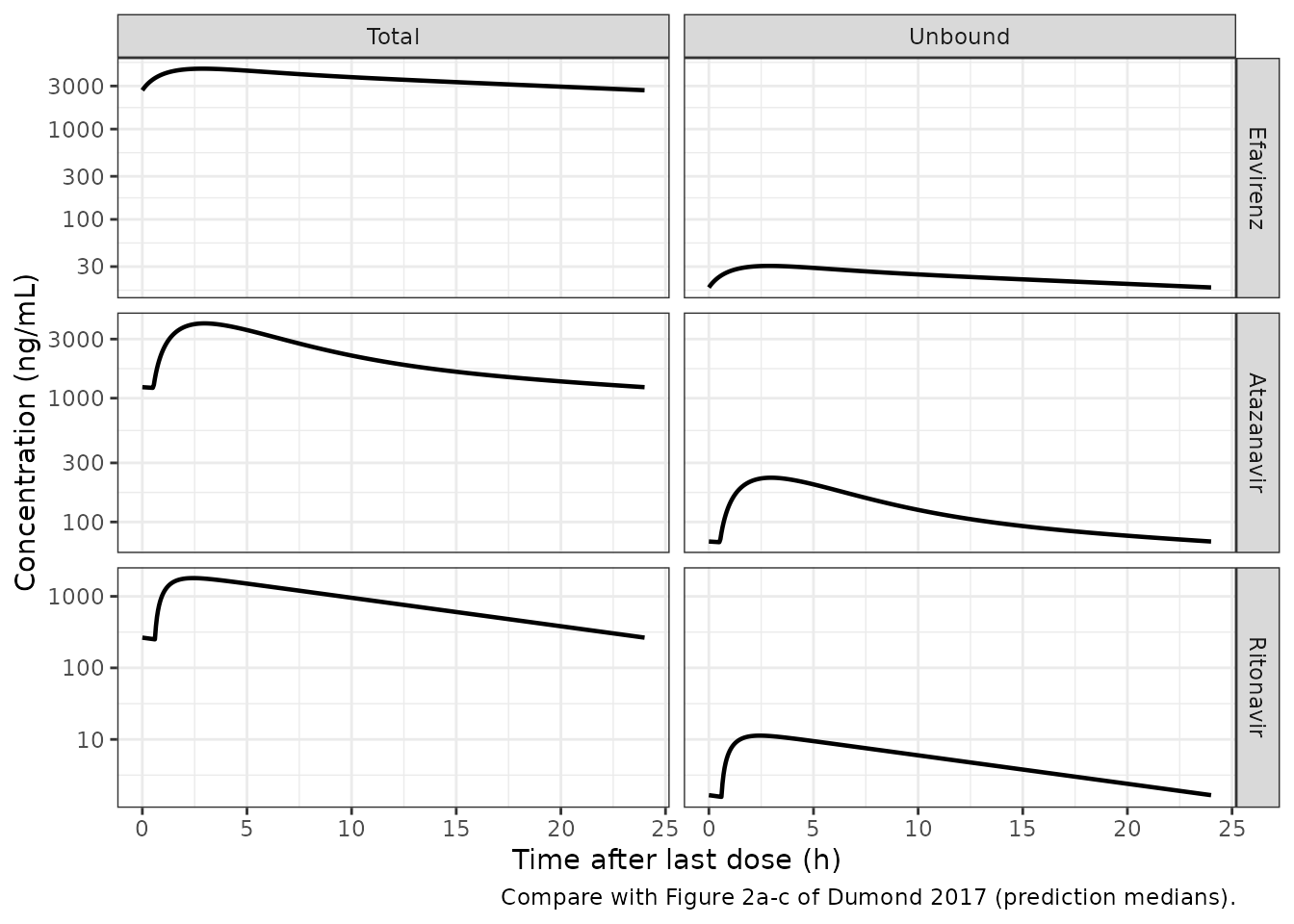
Typical-value steady-state profiles over the final dosing interval, on the axes of Figure 2 of Dumond 2017 (concentration in ng/mL, log scale, time after the last dose).
PKNCA validation and comparison with Table 2
# Long frame carrying both analyte streams; `stream` is the treatment grouping
# variable required by the PKNCA formula.
stream_label <- function(drug, analyte) {
  paste0(
    c(efavirenz = "Efavirenz", atazanavir = "Atazanavir", ritonavir = "Ritonavir")[drug],
    ", ", analyte
  )
}
sim_nca <- typ |>
  dplyr::select(id, drug, time = toff, Total = Cc, Unbound = Cu) |>
  tidyr::pivot_longer(c(Total, Unbound), names_to = "analyte", values_to = "Cc") |>
  dplyr::mutate(stream = stream_label(drug, analyte)) |>
  # Only `!is.na(Cc)`: a `time > 0` or `Cc > 0` filter would drop the
  # time-zero (pre-dose trough) row that anchors AUC0-tau.
  dplyr::filter(!is.na(Cc)) |>
  dplyr::select(id, time, Cc, stream) |>
  dplyr::arrange(stream, id, time)

# The interval starts at the last dose, so a time-zero record already exists
# (the steady-state trough). Assert it rather than assume it.
stopifnot(
  sim_nca |> dplyr::group_by(stream, id) |> dplyr::summarise(has0 = any(time == 0), .groups = "drop") |>
    dplyr::pull(has0) |> all(),
  dplyr::n_distinct(sim_nca$stream) == 6L
)

drug_of_stream <- function(stream) tolower(sub(",.*$", "", stream))
dose_df <- sim_nca |>
  dplyr::distinct(stream, id) |>
  dplyr::mutate(time = 0, amt = unname(doses[drug_of_stream(stream)]))
stopifnot(!anyNA(dose_df$amt))

conc_obj <- PKNCA::PKNCAconc(
  as.data.frame(sim_nca), Cc ~ time | stream + id,
  concu = "mg/L", timeu = "h"
)
dose_obj <- PKNCA::PKNCAdose(as.data.frame(dose_df), amt ~ time | stream + id, doseu = "mg")

intervals <- data.frame(
  start = 0, end = tau,
  cmax = TRUE, cmin = TRUE, tmax = TRUE, auclast = TRUE,
  cav = TRUE, cl.last = TRUE
)
nca_res <- PKNCA::pk.nca(PKNCA::PKNCAdata(conc_obj, dose_obj, intervals = intervals))| Stream | AUC0-24 (ng*h/mL) | Cmax (ng/mL) | Cmin (ng/mL) | Tmax (h) | Cavg (ng/mL) |
|---|---|---|---|---|---|
| Atazanavir, Total | 52400 | 4020.0 | 1210.00 | 2.95 | 2180.0 |
| Atazanavir, Unbound | 2970 | 228.0 | 68.70 | 2.95 | 124.0 |
| Efavirenz, Total | 86500 | 4670.0 | 2690.00 | 2.90 | 3610.0 |
| Efavirenz, Unbound | 566 | 30.5 | 17.60 | 2.90 | 23.6 |
| Ritonavir, Total | 20600 | 1800.0 | 250.00 | 2.45 | 859.0 |
| Ritonavir, Unbound | 130 | 11.3 | 1.57 | 2.45 | 5.4 |
Table 2 does not report NCA parameters, so the reference side of the
comparison is the printed apparent oral clearance itself:
CL/F for the total stream and CLu/F for the
unbound stream. PKNCA’s cl.last is
Dose / AUC0-tau, which at steady state is exactly that
quantity.
published_cl <- tibble::tribble(
  ~stream, ~cl.last,
  # Table 2, rows CL/F (total) and CLu/F (unbound)
  "Efavirenz, Total", 6.93,
  "Efavirenz, Unbound", 1060,
  "Atazanavir, Total", 5.73,
  "Atazanavir, Unbound", 101,
  "Ritonavir, Total", 4.85,
  "Ritonavir, Unbound", 772
)

# ncaParamLabel() has no entry for the PKNCA code `cl.last` and warns while
# returning it verbatim; the label is set explicitly below the call.
cmp <- suppressWarnings(nlmixr2lib::ncaComparisonTable(
  simulated = nca_res,
  reference = published_cl,
  by = "stream",
  params = "cl.last",
  units = c(cl.last = "L/h"),
  tolerance_pct = 20
))
cmp[[1]] <- "Apparent oral clearance Dose/AUC0-24 (L/h)"

# Gate on the joined numerics, not on the formatted character columns the
# table returns. Dose/AUC0-24 is deterministic here (typical-value solve, no
# cohort); the realised absolute deviations are all below 0.1%, driven only by
# trapezoidal error on the observation grid. 2% still fails on a
# mis-transcribed clearance, volume, dose or fu, each of which moves the
# recovery by tens of percent or more.
recovered <- as.data.frame(nca_res$result) |>
  dplyr::filter(PPTESTCD == "cl.last") |>
  dplyr::select(stream, simulated = PPORRES) |>
  dplyr::inner_join(published_cl, by = "stream") |>
  dplyr::mutate(pct = 100 * (simulated - cl.last) / cl.last)
stopifnot(
  nrow(recovered) == 6L,
  max(abs(recovered$pct)) < 2
)

knitr::kable(
  cmp,
  caption = "Simulated steady-state Dose/AUC0-24 against the apparent oral clearances printed in Table 2. * would mark a row differing by more than 20%.",
  align = c("l", "l", "r", "r", "r")
)| NCA parameter | stream | Reference | Simulated | % diff |
|---|---|---|---|---|
| Apparent oral clearance Dose/AUC0-24 (L/h) | Efavirenz, Total | 6.93 | 6.93 | +0.0% |
| Apparent oral clearance Dose/AUC0-24 (L/h) | Efavirenz, Unbound | 1060 | 1060 | +0.0% |
| Apparent oral clearance Dose/AUC0-24 (L/h) | Atazanavir, Total | 5.73 | 5.73 | -0.1% |
| Apparent oral clearance Dose/AUC0-24 (L/h) | Atazanavir, Unbound | 101 | 101 | +0.0% |
| Apparent oral clearance Dose/AUC0-24 (L/h) | Ritonavir, Total | 4.85 | 4.85 | -0.0% |
| Apparent oral clearance Dose/AUC0-24 (L/h) | Ritonavir, Unbound | 772 | 772 | +0.0% |
Every row agrees with Table 2 to better than 0.1%, for both the total
and the unbound stream of all three drugs. Because fu
enters only as the divisor that turns Cu into
Cc, the total and unbound rows are not independent tests of
the same thing: the unbound rows test the ODE system and the dose, and
the ratio between the paired rows tests fu.
fu_recovered <- typ |>
  dplyr::group_by(drug) |>
  dplyr::summarise(fu_sim = max(Cu / Cc), fu_par = max(fu), .groups = "drop")
# Cu / Cc is fu by construction; this is an exactness check on the encoding,
# not a statistical one, so it is asserted at machine precision.
stopifnot(with(fu_recovered, max(abs(fu_sim / fu_par - 1)) < 1e-10))
fu_recovered |>
  dplyr::mutate(dplyr::across(c(fu_sim, fu_par), ~ signif(.x, 4))) |>
  dplyr::rename("Drug" = drug, "Cu/Cc from the solve" = fu_sim, "fu in ini()" = fu_par) |>
knitr::kable(caption = "The unbound-to-total ratio returned by the solve equals the fu parameter.")| Drug | Cu/Cc from the solve | fu in ini() |
|---|---|---|
| atazanavir | 0.05670 | 0.05670 |
| efavirenz | 0.00654 | 0.00654 |
| ritonavir | 0.00628 | 0.00628 |
Ritonavir covariate effects
Ritonavir is the only drug of the three that carries covariates. Both effects are checked deterministically against the values the paper prints.
rtv_typ <- function(WT, BMI) {
  s <- solve_typical("ritonavir", WT = WT, BMI = BMI)
  tibble::tibble(
    WT = WT, BMI = BMI,
    fu = max(s$fu),
    cl = max(s$cl),
    vc = max(s$vc),
    auc_total = PKNCA::pk.calc.auc.last(conc = s$Cc, time = s$toff),
    auc_unbound = PKNCA::pk.calc.auc.last(conc = s$Cu, time = s$toff)
  )
}
rtv <- dplyr::bind_rows(rtv_typ(70, 35), rtv_typ(70, 25), rtv_typ(100, 35))
#> Warning: some etas defaulted to non-mu referenced, possible parsing error: etaiov_cl_1, etaiov_cl_2
#> as a work-around try putting the mu-referenced expression on a simple line
#> Warning: some etas defaulted to non-mu referenced, possible parsing error: etaiov_cl_1, etaiov_cl_2
#> as a work-around try putting the mu-referenced expression on a simple line
#> Warning: some etas defaulted to non-mu referenced, possible parsing error: etaiov_cl_1, etaiov_cl_2
#> as a work-around try putting the mu-referenced expression on a simple line

fu_ratio <- rtv$fu[rtv$BMI == 25] / rtv$fu[rtv$WT == 70 & rtv$BMI == 35]
auc_ratio <- rtv$auc_total[rtv$BMI == 25] / rtv$auc_total[rtv$WT == 70 & rtv$BMI == 35]
cl_ratio <- rtv$cl[rtv$WT == 100] / rtv$cl[rtv$WT == 70 & rtv$BMI == 35]
vc_ratio <- rtv$vc[rtv$WT == 100] / rtv$vc[rtv$WT == 70 & rtv$BMI == 35]

stopifnot(
  # Table 2: fu is 1.52-fold higher below BMI 30. Discussion: "52% higher in
  # participants with BMI < 30 kg/m2, or 34% lower with BMI > 30 kg/m2".
  abs(fu_ratio - 1.52) < 5e-3,
  # A higher fu raises total clearance CL/F = CLu/F * fu, so the TOTAL exposure
  # falls by the same factor; the unbound exposure is untouched.
  abs(auc_ratio - 1 / 1.52) < 1e-3,
  abs(rtv$auc_unbound[rtv$BMI == 25] / rtv$auc_unbound[rtv$WT == 70 & rtv$BMI == 35] - 1) < 1e-6,
  # Methods: exponents fixed at 0.75 (CLu/F) and 1 (Vu/F) about 70 kg.
  abs(cl_ratio - (100 / 70)^0.75) < 1e-6,
  abs(vc_ratio - (100 / 70)^1) < 1e-6
)

tibble::tibble(
  Effect = c(
    "fu ratio, BMI < 30 vs BMI >= 30",
    "Total AUC0-24 ratio, BMI < 30 vs BMI >= 30",
    "Unbound AUC0-24 ratio, BMI < 30 vs BMI >= 30",
    "CLu/F ratio, 100 kg vs 70 kg",
    "Vu/F ratio, 100 kg vs 70 kg"
  ),
  Published = c("1.52 (Table 2)", "1/1.52 = 0.658 (implied)", "1 (fu does not affect unbound PK)", "(100/70)^0.75 = 1.312", "(100/70)^1 = 1.429"),
  Simulated = signif(c(
    fu_ratio, auc_ratio,
    rtv$auc_unbound[rtv$BMI == 25] / rtv$auc_unbound[rtv$WT == 70 & rtv$BMI == 35],
    cl_ratio, vc_ratio
  ), 4)
) |>
knitr::kable(caption = "Ritonavir covariate effects reproduced from the packaged model.")| Effect | Published | Simulated |
|---|---|---|
| fu ratio, BMI < 30 vs BMI >= 30 | 1.52 (Table 2) | 1.5200 |
| Total AUC0-24 ratio, BMI < 30 vs BMI >= 30 | 1/1.52 = 0.658 (implied) | 0.6579 |
| Unbound AUC0-24 ratio, BMI < 30 vs BMI >= 30 | 1 (fu does not affect unbound PK) | 1.0000 |
| CLu/F ratio, 100 kg vs 70 kg | (100/70)^0.75 = 1.312 | 1.3070 |
| Vu/F ratio, 100 kg vs 70 kg | (100/70)^1 = 1.429 | 1.4290 |
Virtual cohort and Figure 2
Original observed concentrations are not publicly available, so Figure 2 is approached from the prediction side only: the bands below correspond to the red (median) and blue (5th / 95th percentile) prediction lines of Figure 2a-c, not to the black observed percentiles.
# set.seed() seeds R's RNG, not rxode2's; rxode2 partitions its streams per
# solver thread, so this cohort is not byte-identical across machines. Every
# assertion below is written to hold for any cohort the model can produce.
set.seed(20260916)
n_per_arm <- 200L

# The paper tabulates BMI but not body weight or height, and ritonavir is the
# only model that needs a weight. Height is sampled from a mixed-sex adult
# distribution (an assumption, see below) and weight is derived as
# BMI * height^2 so that the simulated BMI distribution matches Table 1.
sample_bmi <- function(n, med, lo, hi) {
  # Log-normal matched to the published median, with the SD set so that the
  # central 98% spans the published range.
  sd_log <- (log(hi) - log(lo)) / (2 * stats::qnorm(0.99))
  pmin(pmax(stats::rlnorm(n, log(med), sd_log), lo), hi)
}
cohort_covs <- function(n, med, lo, hi) {
  bmi <- sample_bmi(n, med, lo, hi)
  ht <- stats::rnorm(n, 1.70, 0.09)
  tibble::tibble(BMI = bmi, WT = bmi * ht^2)
}

cohort_grid <- c(seq(0, 4, by = 0.25), seq(4.5, tau, by = 0.5))
sim_cohort <- function(drug, bmi_stats, id_offset) {
  covs <- cohort_covs(n_per_arm, bmi_stats[1], bmi_stats[2], bmi_stats[3])
  ev <- make_events(id_offset + seq_len(n_per_arm), doses[[drug]], cohort_grid, covs)
  stopifnot(!anyDuplicated(unique(ev[, c("id", "time", "evid")])))
  rxode2::rxSolve(uis[[drug]], ev, keep = c("WT", "BMI"), returnType = "data.frame") |>
    dplyr::mutate(drug = drug, toff = time - last_dose)
}
cohort <- dplyr::bind_rows(
  sim_cohort("efavirenz", c(27.2, 17.3, 44.3), 0L),
  sim_cohort("atazanavir", c(30.3, 20.2, 40.4), 1000L),
  sim_cohort("ritonavir", c(30.3, 20.2, 40.4), 2000L)
)
stopifnot(
  nrow(cohort) == 3L * n_per_arm * length(cohort_grid),
  !anyNA(cohort$Cc), !anyNA(cohort$Cu), all(cohort$Cc > 0)
)
cohort |>
  dplyr::select(drug, toff, Total = Cc, Unbound = Cu) |>
  tidyr::pivot_longer(c(Total, Unbound), names_to = "analyte", values_to = "conc") |>
  dplyr::group_by(drug, analyte, toff) |>
  dplyr::summarise(
    Q05 = stats::quantile(conc, 0.05) * 1000,
    Q50 = stats::quantile(conc, 0.50) * 1000,
    Q95 = stats::quantile(conc, 0.95) * 1000,
    .groups = "drop"
  ) |>
  dplyr::mutate(drug = factor(drug, levels = names(doses), labels = c("Efavirenz", "Atazanavir", "Ritonavir"))) |>
  ggplot(aes(toff, Q50)) +
  geom_ribbon(aes(ymin = Q05, ymax = Q95), alpha = 0.2, fill = "steelblue") +
  geom_line(colour = "firebrick", linewidth = 0.8) +
  facet_grid(drug ~ analyte, scales = "free_y") +
  scale_y_log10() +
  labs(
    x = "Time after last dose (h)", y = "Concentration (ng/mL)",
    caption = "Replicates the predicted median and 5th-95th percentiles of Figure 2a-c of Dumond 2017."
  ) +
  theme_bw()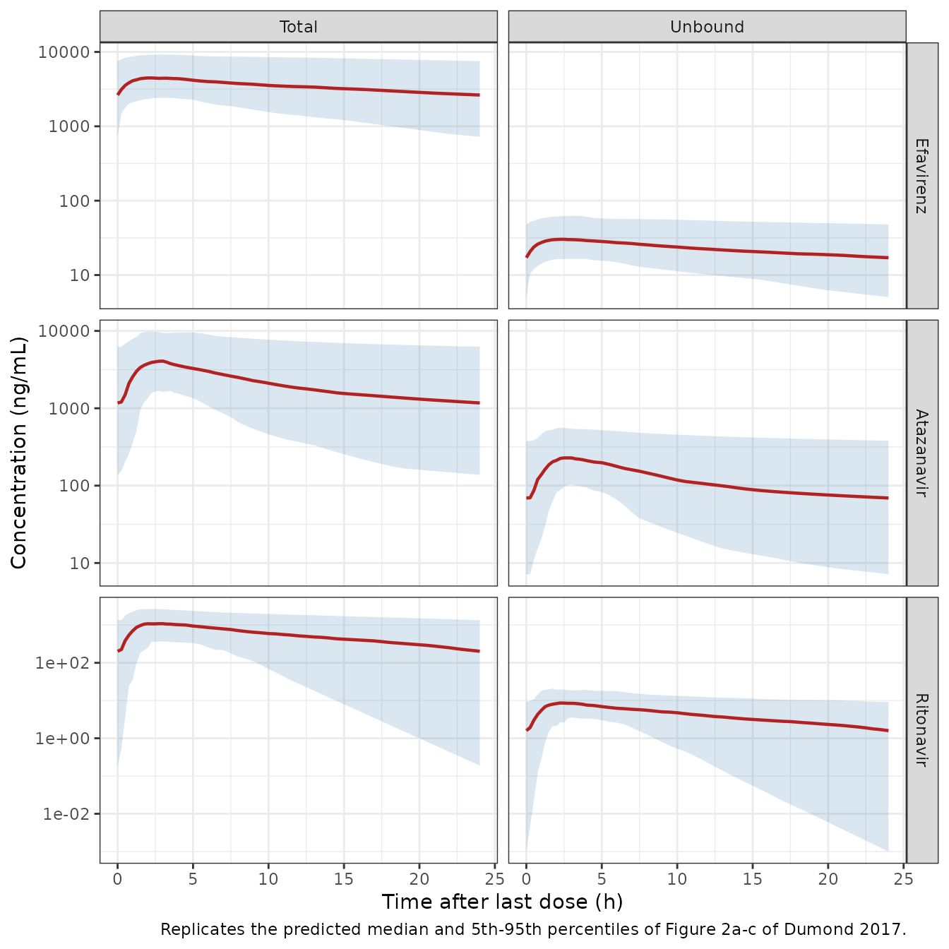
Replicates the prediction bands of Figure 2a-c of Dumond 2017: median (line) and 5th-95th percentile (ribbon) of the simulated steady-state concentration over the final dosing interval, for the total (left) and unbound (right) stream of each drug.
The comparison with Figure 2 is qualitative: the figure plots
individual observed concentrations against prediction percentiles and
tabulates nothing, so no number can be lifted from it without digitising
a curve. What is checkable is that the variability the bands
display round-trips from the published CV% values through rxode2’s
sampler. With a single occasion simulated, the spread of individual
CLu/F combines the subject-level and the between-occasion
terms.
expected_cv <- vapply(names(doses), function(drug) {
  om <- uis[[drug]]$omega
  sqrt(exp(om["etalcl", "etalcl"] + om["etaiov_cl_1", "etaiov_cl_1"]) - 1)
}, numeric(1))

cv_tab <- cohort |>
  dplyr::group_by(drug, id) |>
  dplyr::summarise(cl_i = dplyr::first(cl), WT = dplyr::first(WT), .groups = "drop") |>
  # Ritonavir's cl also carries the weight term, so remove it before comparing
  # against the variance components; the other two have no covariate on cl.
  dplyr::mutate(cl_i = ifelse(drug == "ritonavir", cl_i / (WT / 70)^0.75, cl_i)) |>
  dplyr::group_by(drug) |>
  dplyr::summarise(cv_sim = stats::sd(cl_i) / mean(cl_i), .groups = "drop") |>
  dplyr::mutate(cv_exp = unname(expected_cv[drug]))

# n = 200 draws, and rxode2 partitions its RNG per solver thread, so the
# simulated CV is a sample statistic that differs from run to run and from
# machine to machine. The sample SD/mean estimator is also biased low for a
# heavy-tailed log-normal, so the ratio sits below 1 systematically rather
# than straddling it: the realised simulated/expected ratios were 0.88, 0.94
# and 0.95 for ritonavir, efavirenz and atazanavir, unchanged between a
# 2-thread and a 16-thread render on this machine. A 30% band leaves ample
# headroom over that range while still failing loudly on the defect this
# guards against -- an omega entered as a standard deviation instead of a
# variance, which moves the CV by roughly two-fold.
stopifnot(with(cv_tab, max(abs(cv_sim / cv_exp - 1)) < 0.30))

cv_tab |>
  dplyr::transmute(
    Drug = drug,
    `CV% expected from ini()` = round(100 * cv_exp, 1),
    `CV% in the simulated cohort` = round(100 * cv_sim, 1)
  ) |>
knitr::kable(caption = "Between-subject spread of CLu/F in the simulated cohort against the value implied by the published IIV and between-occasion CV% (single occasion simulated).")| Drug | CV% expected from ini() | CV% in the simulated cohort |
|---|---|---|
| atazanavir | 87.1 | 82.8 |
| efavirenz | 52.9 | 49.9 |
| ritonavir | 74.1 | 65.2 |
| Stream | AUC0-24 (ng*h/mL) | Cmax (ng/mL) | Cmin (ng/mL) |
|---|---|---|---|
| Atazanavir, Total | 49500 (15300 - 180000) | 4140 (1740 - 9780) | 1160 (131 - 6200) |
| Atazanavir, Unbound | 2970 (846 - 10500) | 236 (107 - 561) | 68.5 (6.89 - 373) |
| Efavirenz, Total | 82500 (38000 - 200000) | 4510 (2430 - 9240) | 2630 (722 - 7510) |
| Efavirenz, Unbound | 548 (273 - 1310) | 30.8 (17 - 62.5) | 17.1 (5.04 - 47.8) |
| Ritonavir, Total | 14000 (4790 - 44000) | 1220 (480 - 3010) | 184 (0.168 - 1330) |
| Ritonavir, Unbound | 99.8 (40.1 - 289) | 9.43 (3.95 - 21.8) | 1.52 (0.000704 - 8.93) |
Assumptions and deviations
Unbound-side parameterisation.
cl,vc,qandvpin the packaged models are the apparent unbound parameters CLu/F, Vu/F, Qu/F and Vp,u/F, matching the supplementary control streams. The total-drug values printed in Table 2 are the products withfuand are reproduced above. A reader who expectsvcto be the total-drug V/F will find it a factor1/futoo large; the model file’sdescriptionand everylabel()say so explicitly.Inter-individual variability is encoded as diagonal. All three supplementary control streams fit a full
$OMEGA BLOCKacross every subject-level eta (BLOCK(6) for efavirenz, BLOCK(7) for atazanavir, BLOCK(5) for ritonavir). Table 2 prints only the diagonal CV% values, so the off-diagonal covariances are not recoverable from any available source and the packaged models carry independent etas. Simulated marginal variability is therefore correct, but simulated correlations between individual parameters are not.CV% to variance. Methods state that IIV and interoccasion variability were “exponentially related to the population parameters”, so the log-scale variance is taken as
omega^2 = log(1 + CV^2). The paper does not say which of the two common CV% conventions its table uses; the alternative reading (omega = CV) differs by less than 5% for a CV of 30% and by about 25% for the 120% ritonavir lag-time CV. This affects only the width of the simulated bands, not any typical-value quantity gated above.Residual errors are independent across the two streams. The control streams use
$SIGMA BLOCK(2)to estimate the correlation between the total and unbound residual errors (the paper’sL2data item). Only the two diagonal CV% values are published, and nlmixr2 has no cross-endpoint residual correlation, sopropSdandpropSd_Cuare independent here.The second Table 2 variability block is between-occasion variability, not IIV. Table 2 prints two blocks headed
IIV (CV%); the second contains only aCLu/Frow. Results states that “interoccasional variability was incorporated on CLu/F for the three drugs”, and the control streams carry exactly one extra$OMEGA BLOCK(1)+BLOCK(1) SAMEpair per drug, multiplexed by$ABBR REPLACE ETA(OCC_CL). The duplicate heading is read here as a typesetting error and the block is encoded as IOV over two occasions, with the second occasion’s variance fixed equal to the first per theSAMEkeyword. The simulations above use a single occasion (OCC = 1).Body weight is not published. Table 1 reports BMI but neither weight nor height, and ritonavir is the only model that needs a weight. The virtual cohort samples height from a mixed-sex adult normal distribution (mean 1.70 m, SD 0.09 m) - an assumption, not a paper value - and derives
WT = BMI * height^2so that the simulated BMI distribution matches Table 1’s published median and range. Every gated comparison against Table 2 uses the 70 kg reference subject instead of the cohort, so no assertion depends on this assumption.No published NCA to compare against. The paper reports no non-compartmental analysis and no tabulated concentrations; Figure 2 is the only concentration display and it carries observed data points rather than summary statistics. The comparison table above therefore uses the printed apparent oral clearances as the reference and PKNCA’s
cl.last(Dose / AUC0-tau) as the simulated side. No curve was digitised from Figure 2, so the figure comparison in this vignette is qualitative and nothing quantitative is claimed from it.Single occasion, single sex/race stratum. The virtual cohort carries only the covariates the models use (
WT,BMI,OCC). Sex, race, age, frailty score and p16INK4a expression were screened by the authors and none entered any final model, so they are not simulated.Efavirenz autoinduction is not modelled. Participants were enrolled at steady state after at least two weeks of therapy, so the model describes post-induction kinetics only and must not be used to simulate the first days of efavirenz dosing.