Ceftaroline in critically ill adults with and without CRRT (Adamiszak 2025)
Source:vignettes/articles/Adamiszak_2025_ceftaroline.Rmd
Adamiszak_2025_ceftaroline.RmdModel and source
- Citation: Adamiszak A, Pietrzkiewicz K, Bartkowska-Sniatkowska A, Smuszkiewicz P, Kusza K, Grzeskowiak E, Bienert A (2025). Do Critically Ill Patients Undergoing Continuous Renal Replacement Therapy Require Ceftaroline Dosage Adjustments? Ceftaroline PopPK Model and Dosage Simulations with the Probability of Target Attainment Analysis Based on Retrospective Data. Antibiotics 14(4):347. doi:10.3390/antibiotics14040347.
- Description: Five-compartment population PK model for ceftaroline in critically ill adults with and without continuous renal replacement therapy (CRRT): a two-compartment patient model (first-order elimination from the central, pre-filter compartment) joined to three CRRT-machine compartments (filter, post-filter return limb and effluent) whose transfer rate constants are circuit flow divided by compartment volume, all gated on by a time-varying CRRT-running indicator. Creatinine clearance (power model centred at 159 mL/min/1.73 m^2) on clearance; CRRT modality (CVVHD, CVVHDF) on the central volume; any CRRT on the peripheral volume and intercompartmental clearance. Between-occasion variability on clearance, between-subject variability on the central and peripheral volumes and intercompartmental clearance, and proportional residual error for each of the three sampled matrices (systemic pre-filter plasma, post-filter plasma, effluent).
- Article: https://doi.org/10.3390/antibiotics14040347
- Supplement (final-model mlxtran syntax, Table S1): https://www.mdpi.com/article/10.3390/antibiotics14040347/s1
- Authors’ Simulx 2024R1 project and PTA workbooks: https://github.com/arkadiusz-adamiszak/Ceftaroline_ICU_Retrospective
mod <- readModelDb("Adamiszak_2025_ceftaroline")
ui <- rxode2::rxode(mod)
#> ℹ parameter labels from comments will be replaced by 'label()'
#> Warning: some etas defaulted to non-mu referenced, possible parsing error: etaiov_cl_1, etaiov_cl_2
#> as a work-around try putting the mu-referenced expression on a simple line
mod_typ <- rxode2::zeroRe(ui)
#> Warning: some etas defaulted to non-mu referenced, possible parsing error: etaiov_cl_1, etaiov_cl_2
#> as a work-around try putting the mu-referenced expression on a simple line
th <- ui$theta
The model joins a two-compartment patient model to three compartments
that stand for the CRRT machine, following the cefepime structure of
Al-Shaer et al. that the paper cites (Figure 1). Blood leaves the
patient’s central (pre-filter) compartment at the blood flow rate
Qb into the filter (circuit_plasma, volume
VCRRT). From the filter, drug passes at Qb
into the post-filter return limb (circuit_postfilter),
which returns it to the patient at Qb, and at the effluent
flow rate Qeff into the effluent compartment
(circuit_dialysate), which washes out at Qeff.
Every transfer rate constant is flow / volume (Methods 4.2). All circuit
terms are multiplied by the time-varying indicator
RRT_CRRT_ACTIVE (the mlxtran regressor
IS_CRRT), so a patient whose CRRT is stopped reverts to the
two-compartment model.
The paper’s Figure 1 calls the last compartment “Effluent”. It is
carried here as circuit_dialysate, not
circuit_effluent, because drug flows through it and out at
Qeff; circuit_effluent is the accumulating
waste bag, from which nothing leaves. Its concentration is the effluent
assay (Ceffluent).
Population
Adamiszak 2025 pooled concentrations from four published studies of critically ill adults receiving 400-600 mg of ceftaroline fosamil every 8-12 h as a 1 h infusion (Alarcia-Lacalle 2021, Chauzy 2019, Chauzy 2022, Kalaria 2021). The concentrations were digitised from those papers’ figures with WebPlotDigitizer 4.7: 296 plasma concentrations from 29 patients not on CRRT, and 24 pre-filter (systemic), 23 post-filter and 23 effluent concentrations from 4 patients on CRRT. Table 1 gives the 33 patients as 36% female, median age 51 years (range 21-77), median weight 75.5 kg (49-111.8) and median MDRD creatinine clearance 159 mL/min/1.73 m^2 (42-309). Of the four CRRT patients two were on CVVHD and two on CVVHDF, with blood flow 250 [250-300] mL/min and effluent flow 3200 [2700-3660] mL/h.
The same information is available programmatically via
readModelDb("Adamiszak_2025_ceftaroline")()$population.
Source trace
Every ini() value carries an in-file comment naming its
source. Table 2 of the article is mis-rendered in the HTML version; the
values below were read from the PDF layout.
| Equation / parameter | Value | Source location |
|---|---|---|
ODE system, outputs, dosing into Acent
|
– | Supplement, “Monolix model syntax”; identical to
ModelFile/Syntax_v2_SameClbody+IS_CRRT+Q.txt in the
authors’ Simulx project |
Transfer rate constant k = flow / V
|
– | Methods 4.2 equation |
Continuous covariate (COV / median COV)^theta
|
– | Methods 4.2 equation; median 159 from Table 1 (Simulx
logtClCr_Pros = log(ClCr_Pros/159)) |
Categorical covariate exp(theta)
|
– | Methods 4.2 equation |
| Modality on VCentral, any-CRRT on VPeripheral and Q, no-CRRT reference | – | Results 2.2; Simulx covariate definitions
tCRRT_NaRef_CVVHD_CVVHDF,
tCRRT_NaRef_CRRT
|
lcl (Cl) |
11.23 L/h | Table 2, Final Model |
e_crcl_cl |
0.68 | Table 2 |
lvc (VCentral) |
20.04 L | Table 2 |
e_cvvhd_vc, e_cvvhdf_vc
|
0.47, -0.42 | Table 2 |
lq (Q), e_crrt_q
|
8.80 L/h, 0.99 | Table 2 |
lvp (VPeripheral), e_crrt_vp
|
16.85 L, 0.99 | Table 2 |
lvfilter (VCRRT) |
2.69 L | Table 2 |
lvpostfilter (VPost-filter) |
1.15 L | Table 2 |
lvdialysate (VEffluent) |
0.60 L | Table 2 |
etaiov_cl_1, etaiov_cl_2
|
IOV 34.96% CV | Table 2 |
etalvc, etalq, etalvp
|
IIV 3.70, 16.40, 38.60% CV | Table 2 |
propSd, propSd_Cpostfilter,
propSd_Ceffluent
|
0.29, 0.16, 0.13 | Table 2 (bPre, bPost, bEff) |
| Free fraction 0.8 for PTA | – | Methods 4.3 (~20% protein binding); Simulx
FreeCcent = 0.8*Ccent
|
Simulation helpers
Dose rows go into the central state; observation rows
carry dvid = 1 and no compartment, so all three outputs
(Cc, Cpostfilter, Ceffluent) are
returned at every observation time. The CRRT flows are supplied in the
units the covariate register uses, blood flow in mL/min and effluent
flow in mL/h.
# One subject's dosing + observation records. crrt is one of "none", "CVVHD",
# "CVVHDF"; qeff_lh is the effluent flow in L/h, converted to mL/h on the
# record.
make_events <- function(dose, tau, tinf, ndose, obs_times, crcl, crrt = "none",
                        qeff_lh = 0, bfr = 250) {
  doses <- data.frame(
    time = (seq_len(ndose) - 1) * tau, amt = dose, rate = dose / tinf,
    evid = 1L, cmt = "central", dvid = NA_integer_
  )
  obs <- data.frame(
    time = obs_times, amt = NA_real_, rate = NA_real_,
    evid = 0L, cmt = NA_character_, dvid = 1L
  )
  ev <- rbind(doses, obs)
  ev <- ev[order(ev$time, -ev$evid), ]
  on <- as.numeric(crrt != "none")
  ev$CRCL <- crcl
  ev$RRT_CVVHD_STATUS <- as.numeric(crrt == "CVVHD")
  ev$RRT_CVVHDF_STATUS <- as.numeric(crrt == "CVVHDF")
  ev$RRT_CRRT_ACTIVE <- on
  ev$BFR <- bfr * on
  ev$RRT_CRRT_EFFLUENT_FLOW <- qeff_lh * 1000 * on
  ev$OCC <- 1L
  ev
}

replicate_ids <- function(ev, n) {
  out <- ev[rep(seq_len(nrow(ev)), times = n), ]
  out$id <- rep(seq_len(n), each = nrow(ev))
  out
}

# The authors' Simulx target-attainment rule, reproduced exactly below: the
# free concentration is sampled hourly from 0 to 120 h, and the target counts
# as attained when at least 100 of the 120 one-hour intervals have BOTH
# endpoints at or above the MIC.
attained <- function(conc, mic) {
  above <- conc >= mic
  sum(above[-1] & above[-length(above)]) >= 100
}

pta_by_mic <- function(sim, mics) {
  free <- split(0.8 * sim$Cc, sim$id)
  vapply(mics, function(m) mean(vapply(free, attained, logical(1), mic = m)), numeric(1))
}
Typical-value checks against the paper’s own numbers
The Results and Discussion quote several derived quantities. Each is recomputed from the packaged parameters.
cl_at <- function(crcl) exp(th[["lcl"]]) * (crcl / 159)^th[["e_crcl_cl"]]
anchors <- tibble::tribble(
  ~quantity, ~paper, ~model,
  "Cl, non-CRRT median patient (L/h), Discussion", 11.2, cl_at(159),
  "Cl, CRRT simulation patient CrCL 58 (L/h), Discussion", 5.66, cl_at(58),
  "Cl at CrCL 309 vs 159 (ratio), Results: +57%", 1.57, cl_at(309) / cl_at(159),
  "VCentral on CVVHD vs no CRRT (ratio), Results: +60%", 1.60, exp(th[["e_cvvhd_vc"]]),
  "VPeripheral and Q on CRRT vs no CRRT (ratio)", 2.69, exp(th[["e_crrt_vp"]])
)
anchors |>
  mutate(model = signif(model, 4), pct_diff = round(100 * (model / paper - 1), 2)) |>
knitr::kable()| quantity | paper | model | pct_diff |
|---|---|---|---|
| Cl, non-CRRT median patient (L/h), Discussion | 11.20 | 11.230 | 0.27 |
| Cl, CRRT simulation patient CrCL 58 (L/h), Discussion | 5.66 | 5.657 | -0.05 |
| Cl at CrCL 309 vs 159 (ratio), Results: +57% | 1.57 | 1.571 | 0.06 |
| VCentral on CVVHD vs no CRRT (ratio), Results: +60% | 1.60 | 1.600 | 0.00 |
| VPeripheral and Q on CRRT vs no CRRT (ratio) | 2.69 | 2.691 | 0.04 |
All five agree to the precision printed. The decisive one is the CRRT patient’s 5.66 L/h: it fixes the clearance, the exponent and the centring value 159 simultaneously, and the centring value is never stated in the text.
Circuit clearance at steady state
Because every circuit transfer is linear, at steady state the filter
concentration is Qb / (Qb + Qeff) times the systemic
concentration and the effluent removes drug at Qeff times
that. The total clearance seen by the systemic compartment is therefore
Cl + Qb * Qeff / (Qb + Qeff), which must equal dose / AUC
over a dosing interval. The solve below checks that identity for a
typical patient off CRRT and on each modality.
qb_lh <- 250 * 60 / 1000
ss_cases <- tibble::tribble(
  ~case, ~crcl, ~crrt, ~qeff,
  "No CRRT, CrCL 159", 159, "none", 0,
  "CVVHD, CrCL 58, Qeff 2.5 L/h", 58, "CVVHD", 2.5,
  "CVVHDF, CrCL 58, Qeff 4.0 L/h", 58, "CVVHDF", 4.0
)
ss_rows <- lapply(seq_len(nrow(ss_cases)), function(i) {
  ev <- make_events(600, 12, 1, 20, seq(216, 228, by = 0.02),
    crcl = ss_cases$crcl[i], crrt = ss_cases$crrt[i], qeff_lh = ss_cases$qeff[i]
  )
  s <- as.data.frame(rxode2::rxSolve(mod_typ, ev, returnType = "data.frame"))
  auc <- sum(diff(s$time) * (head(s$Cc, -1) + tail(s$Cc, -1)) / 2)
  expected <- cl_at(ss_cases$crcl[i]) +
    if (ss_cases$qeff[i] > 0) qb_lh * ss_cases$qeff[i] / (qb_lh + ss_cases$qeff[i]) else 0
  data.frame(case = ss_cases$case[i], dose_over_auc = 600 / auc, expected = expected)
})
#> ℹ omega/sigma items treated as zero: 'etaiov_cl_1', 'etaiov_cl_2', 'etalvc', 'etalq', 'etalvp'
#> ℹ omega/sigma items treated as zero: 'etaiov_cl_1', 'etaiov_cl_2', 'etalvc', 'etalq', 'etalvp'
#> ℹ omega/sigma items treated as zero: 'etaiov_cl_1', 'etaiov_cl_2', 'etalvc', 'etalq', 'etalvp'
ss_tab <- bind_rows(ss_rows) |> mutate(pct_diff = 100 * (dose_over_auc / expected - 1))
ss_tab |> mutate(across(where(is.numeric), \(x) signif(x, 4))) |> knitr::kable()| case | dose_over_auc | expected | pct_diff |
|---|---|---|---|
| No CRRT, CrCL 159 | 11.230 | 11.230 | -1.23e-05 |
| CVVHD, CrCL 58, Qeff 2.5 L/h | 7.800 | 7.800 | -1.10e-06 |
| CVVHDF, CrCL 58, Qeff 4.0 L/h | 8.815 | 8.815 | -4.30e-06 |
The Discussion describes total clearance on CRRT as “5.66 L/h +
assumed Qeff”. The model’s actual circuit clearance is
slightly smaller than Qeff (2.14 rather than 2.5 L/h at
Qeff 2.5 L/h), because only the fraction
Qb / (Qb + Qeff) of the drug entering the filter reaches
the effluent side.
Interrupting CRRT (Figure 5)
Figure 5 simulates 600 mg every 12 h as a 1 h infusion in a CVVHD
patient whose effluent flow is 2.5 L/h, with CRRT stopped for 24 h at 48
h and restarted at 4.0 L/h (the Simulx regressor schedule
Real_Time: times 0, 48 and 72 h). The covariates change on
a dense grid so the solver cannot step over the switch.
grid5 <- seq(0, 120, by = 0.1)
ev5 <- make_events(600, 12, 1, 10, grid5, crcl = 58, crrt = "CVVHD", qeff_lh = 2.5)
off <- ev5$time >= 48 & ev5$time < 72
ev5$RRT_CRRT_ACTIVE[off] <- 0
ev5$BFR[off] <- 0
ev5$RRT_CRRT_EFFLUENT_FLOW[off] <- 0
ev5$RRT_CRRT_EFFLUENT_FLOW[ev5$time >= 72] <- 4000
sim5 <- as.data.frame(rxode2::rxSolve(mod_typ, ev5, returnType = "data.frame"))
#> ℹ omega/sigma items treated as zero: 'etaiov_cl_1', 'etaiov_cl_2', 'etalvc', 'etalq', 'etalvp'

sim5 |>
  select(time, Cc, Cpostfilter, Ceffluent) |>
  pivot_longer(-time, names_to = "output", values_to = "conc") |>
  ggplot(aes(time, conc, colour = output)) +
  geom_line() +
  geom_vline(xintercept = c(48, 72), linetype = "dashed") +
  labs(
    x = "Time (h)", y = "Ceftaroline (mg/L)", colour = NULL,
    title = "Replicates Figure 5 of Adamiszak 2025",
    subtitle = "Typical CVVHD patient, CrCL 58; CRRT off from 48 to 72 h"
  )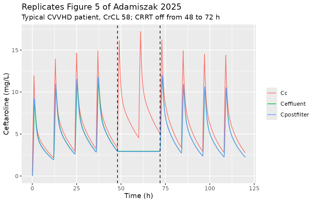
While the circuit is stopped its compartments are frozen: no flow enters or leaves them, so the effluent concentration holds at its 48 h value. The systemic trough rises because the circuit clearance is gone.
frozen <- sim5$Ceffluent[sim5$time > 48.05 & sim5$time < 71.95]
trough <- function(t) sim5$Cc[which.min(abs(sim5$time - t))]
stopifnot(
  diff(range(frozen)) < 1e-6 * max(frozen),
  trough(72) > trough(48)
)
c(trough_48h = trough(48), trough_72h = trough(72), effluent_frozen = frozen[1])
#>      trough_48h      trough_72h effluent_frozen
#>        3.330282        5.045000        2.955091
Virtual cohort and NCA
The paper reports no NCA. The cohort below gives the steady-state
exposure the model implies for 600 mg every 12 h (1 h infusion) in four
groups of 200: off CRRT at CrCL 80 and at the median 159 mL/min/1.73
m^2, and on CVVHD or CVVHDF at CrCL 58 with Qeff 3.0 L/h.
NCA uses the tenth dosing interval (108-120 h).
n_arm <- 200
arms <- tibble::tribble(
  ~treatment, ~crcl, ~crrt, ~qeff,
  "No CRRT, CrCL 80", 80, "none", 0,
  "No CRRT, CrCL 159", 159, "none", 0,
  "CVVHD, Qeff 3.0", 58, "CVVHD", 3.0,
  "CVVHDF, Qeff 3.0", 58, "CVVHDF", 3.0
)
obs_nca <- sort(unique(c(0, seq(108, 120, by = 0.25))))
rxode2::rxSetSeed(20250327)
cohort <- bind_rows(lapply(seq_len(nrow(arms)), function(i) {
  ev <- replicate_ids(make_events(600, 12, 1, 11, obs_nca,
    crcl = arms$crcl[i], crrt = arms$crrt[i], qeff_lh = arms$qeff[i]
  ), n_arm)
  s <- as.data.frame(rxode2::rxSolve(mod, ev, returnType = "data.frame"))
  s$treatment <- arms$treatment[i]
  s
}))
#> ℹ parameter labels from comments will be replaced by 'label()'
#> Warning: some etas defaulted to non-mu referenced, possible parsing error: etaiov_cl_1, etaiov_cl_2
#> as a work-around try putting the mu-referenced expression on a simple line

conc <- cohort |>
  filter(!is.na(Cc)) |>
  select(id, time, Cc, treatment)
dose <- bind_rows(lapply(arms$treatment, function(tr) {
  data.frame(id = rep(seq_len(n_arm), each = 11), time = rep((0:10) * 12, n_arm), amt = 600, treatment = tr)
}))
conc_obj <- PKNCA::PKNCAconc(conc, Cc ~ time | treatment + id, concu = "mg/L", timeu = "h")
dose_obj <- PKNCA::PKNCAdose(dose, amt ~ time | treatment + id, doseu = "mg")
intervals <- data.frame(start = 120 - 12, end = 120, cmax = TRUE, cmin = TRUE, auclast = TRUE)
nca <- PKNCA::pk.nca(PKNCA::PKNCAdata(conc_obj, dose_obj, intervals = intervals))
nca_tab <- as.data.frame(nca$result) |>
  filter(PPTESTCD %in% c("cmax", "cmin", "auclast")) |>
  group_by(treatment, PPTESTCD) |>
  summarise(median = median(PPORRES), p05 = quantile(PPORRES, 0.05), p95 = quantile(PPORRES, 0.95), .groups = "drop")
nca_tab |>
  mutate(across(where(is.numeric), \(x) signif(x, 3))) |>
  rename("NCA parameter" = PPTESTCD) |>
knitr::kable()| treatment | NCA parameter | median | p05 | p95 |
|---|---|---|---|---|
| CVVHD, Qeff 3.0 | auclast | 75.500 | 46.500 | 106.00 |
| CVVHD, Qeff 3.0 | cmax | 15.000 | 12.300 | 17.70 |
| CVVHD, Qeff 3.0 | cmin | 3.200 | 1.320 | 5.41 |
| CVVHDF, Qeff 3.0 | auclast | 72.900 | 48.700 | 102.00 |
| CVVHDF, Qeff 3.0 | cmax | 20.400 | 17.000 | 23.40 |
| CVVHDF, Qeff 3.0 | cmin | 2.420 | 1.040 | 4.51 |
| No CRRT, CrCL 159 | auclast | 55.500 | 34.300 | 98.30 |
| No CRRT, CrCL 159 | cmax | 20.200 | 17.300 | 24.60 |
| No CRRT, CrCL 159 | cmin | 0.809 | 0.140 | 2.80 |
| No CRRT, CrCL 80 | auclast | 86.000 | 47.200 | 144.00 |
| No CRRT, CrCL 80 | cmax | 23.200 | 19.400 | 27.80 |
| No CRRT, CrCL 80 | cmin | 2.220 | 0.437 | 5.58 |
AUC over a steady-state interval depends only on the total clearance,
so its median must sit at
dose / (typical Cl + circuit clearance); between-subject
spread in the volumes and Q does not move it.
auc_check <- nca_tab |>
  filter(PPTESTCD == "auclast") |>
  left_join(arms, by = "treatment") |>
  mutate(
    cl_total = cl_at(crcl) + ifelse(qeff > 0, qb_lh * qeff / (qb_lh + qeff), 0),
    expected = 600 / cl_total,
    pct_diff = 100 * (median / expected - 1)
  )
auc_check |> select(treatment, median, expected, pct_diff) |>
mutate(across(where(is.numeric), \(x) signif(x, 3))) |> knitr::kable()| treatment | median | expected | pct_diff |
|---|---|---|---|
| CVVHD, Qeff 3.0 | 75.5 | 73.6 | 2.650 |
| CVVHDF, Qeff 3.0 | 72.9 | 73.6 | -0.861 |
| No CRRT, CrCL 159 | 55.5 | 53.4 | 3.810 |
| No CRRT, CrCL 80 | 86.0 | 85.2 | 0.871 |
Probability of target attainment
The authors’ Simulx project and PTA workbooks are deposited with the paper. They were run with a parameter set that differs from the published Table 2 (see Assumptions and deviations), so this section first reproduces the deposit with the deposit’s own parameters, which tests the model’s structure and the authors’ target-attainment rule, and then shows what Table 2 implies.
Reproducing the deposited simulation, subject by subject
The Simulx project stores the individual parameters of every simulated patient and whether each attained 100% fT>MIC. The 50 patients of the first replicate (no CRRT, CrCL 80, the same patients in all ten regimens) are embedded below, together with their outcomes at five MICs; each is re-solved with the packaged ODE system with covariate effects neutralised so the individual values enter unchanged.
# Simulx project, Simulation/individualParameters.txt, rep 1, group
# 200mg_12h_1h (identical in every group); Vcrrt, Vpost and Veff are constant.
deposit_indiv <- data.frame(
  cl = c(6.4961794, 4.662855, 7.4240015, 3.8788189, 5.8942644, 10.817915, 6.0281723, 8.1881701, 5.1236503, 15.195177, 7.2456477, 7.7380762, 7.6639258, 10.172442, 5.6749265, 9.1180561, 10.52485, 8.2013931, 3.9015253, 9.6435158, 7.2002555, 7.1088918, 5.3512294, 9.6353486, 4.8387506, 9.020375, 8.6931984, 3.6304658, 8.4863661, 10.103719, 6.1315362, 4.5984642, 6.2725378, 4.0911669, 13.006448, 4.584552, 5.6993418, 8.2255944, 7.0115528, 5.66695, 6.6143811, 6.3230041, 7.3387383, 9.0297494, 6.8274751, 4.9305876, 4.1924907, 5.1088857, 6.3929459, 10.486686),
  vc = c(17.517099, 20.06928, 17.789941, 20.309148, 18.878148, 21.110847, 17.994143, 19.656911, 20.671644, 17.616616, 18.785646, 19.910304, 20.659127, 21.565209, 19.130513, 18.797654, 18.720116, 21.568991, 20.477434, 22.674459, 21.126418, 19.722911, 17.888304, 18.360435, 21.753535, 20.530853, 19.235181, 19.488572, 18.414684, 18.21322, 20.120523, 23.422876, 19.133384, 21.155923, 21.70151, 18.118647, 22.279828, 20.199647, 21.138882, 19.903336, 21.066787, 17.910571, 20.013432, 17.637206, 18.607206, 21.274346, 21.232958, 18.724435, 19.75982, 16.609326),
  vp = c(14.751305, 10.292979, 15.786613, 16.315114, 5.0930563, 18.797139, 16.018509, 10.879837, 19.357267, 28.453531, 22.82975, 18.805903, 17.786848, 14.1145, 12.084895, 12.536435, 30.952588, 23.848388, 11.200077, 16.047077, 17.591019, 12.02733, 13.113841, 13.019271, 13.255965, 9.491153, 13.473767, 13.538015, 27.630161, 15.606442, 12.884037, 10.826067, 23.497408, 14.983165, 12.206697, 10.708366, 6.9206913, 18.738555, 23.161132, 10.105402, 12.401239, 15.867724, 15.763941, 24.226245, 19.134211, 12.782613, 14.821284, 14.939544, 18.159728, 20.881435),
  q = c(9.0095658, 7.9024139, 10.00919, 7.6878717, 8.2277892, 8.4397031, 8.4550573, 5.97621, 7.2880863, 8.3484842, 8.9671843, 8.1078035, 6.4960869, 9.1665907, 7.9767893, 9.6640974, 9.1255323, 7.8129333, 7.3058127, 7.5533867, 7.3251212, 6.5917457, 7.6686488, 8.1377737, 7.7371678, 9.2769543, 8.4900937, 6.9668873, 9.2664163, 8.4193413, 8.2911208, 7.589762, 7.0086952, 9.9544229, 7.6250764, 7.5695791, 9.0787738, 9.1749376, 7.7809058, 9.2931385, 8.197149, 7.8385202, 8.1678028, 9.0625337, 7.348901, 6.9044172, 7.8726294, 7.9717164, 9.3437781, 8.4869314)
)
deposit_outcome <- tibble::tribble(
  ~regimen, ~mic, ~attained,
  "200mg_12h_1h", 0.25, "11111011101110111111111010111011110111111111111110",
  "300mg_12h_1h", 0.25, "11111111101111111111111111111111110111111111111111",
  "400mg_12h_1h", 0.25, "11111111111111111111111111111111110111111111111111",
  "600mg_12h_1h", 0.25, "11111111111111111111111111111111111111111111111111",
  "800mg_12h_1h", 0.25, "11111111111111111111111111111111111111111111111111",
  "200mg_8h_2h", 0.25, "11111111111111111111111111111111111111111111111111",
  "300mg_8h_2h", 0.25, "11111111111111111111111111111111111111111111111111",
  "400mg_8h_2h", 0.25, "11111111111111111111111111111111111111111111111111",
  "600mg_8h_2h", 0.25, "11111111111111111111111111111111111111111111111111",
  "800mg_8h_2h", 0.25, "11111111111111111111111111111111111111111111111111",
  "200mg_12h_1h", 0.5, "11011010101000100010101010010011110110111100111110",
  "300mg_12h_1h", 0.5, "11111010101110100110111010011011110111111111111110",
  "400mg_12h_1h", 0.5, "11111011101110111111111010111011110111111111111110",
  "600mg_12h_1h", 0.5, "11111111101111111111111111111111110111111111111111",
  "800mg_12h_1h", 0.5, "11111111111111111111111111111111110111111111111111",
  "200mg_8h_2h", 0.5, "11111111101111111111111111111111110111111111111111",
  "300mg_8h_2h", 0.5, "11111111111111111111111111111111111111111111111111",
  "400mg_8h_2h", 0.5, "11111111111111111111111111111111111111111111111111",
  "600mg_8h_2h", 0.5, "11111111111111111111111111111111111111111111111111",
  "800mg_8h_2h", 0.5, "11111111111111111111111111111111111111111111111111",
  "200mg_12h_1h", 1, "01010000100000000010000010010001010100000000011000",
  "300mg_12h_1h", 1, "01010010100000100010001010010001110110010000011110",
  "400mg_12h_1h", 1, "11011010101000100010101010010011110110111100111110",
  "600mg_12h_1h", 1, "11111010101110100110111010011011110111111111111110",
  "800mg_12h_1h", 1, "11111011101110111111111010111011110111111111111110",
  "200mg_8h_2h", 1, "11111010101110100110111010011011110111111110111110",
  "300mg_8h_2h", 1, "11111011101111111111111011111011110111111111111110",
  "400mg_8h_2h", 1, "11111111101111111111111111111111110111111111111111",
  "600mg_8h_2h", 1, "11111111111111111111111111111111111111111111111111",
  "800mg_8h_2h", 1, "11111111111111111111111111111111111111111111111111",
  "200mg_12h_1h", 2, "00000000000000000000000000000000000000000000000000",
  "300mg_12h_1h", 2, "00010000000000000010000000010000010000000000001000",
  "400mg_12h_1h", 2, "01010000100000000010000010010001010100000000011000",
  "600mg_12h_1h", 2, "01010010100000100010001010010001110110010000011110",
  "800mg_12h_1h", 2, "11011010101000100010101010010011110110111100111110",
  "200mg_8h_2h", 2, "01010000100000000010000010010001010100000000011100",
  "300mg_8h_2h", 2, "11011010100000100010001010010011110110111100111110",
  "400mg_8h_2h", 2, "11111010101110100110111010011011110111111110111110",
  "600mg_8h_2h", 2, "11111011101111111111111011111011110111111111111110",
  "800mg_8h_2h", 2, "11111111101111111111111111111111110111111111111111",
  "200mg_12h_1h", 4, "00000000000000000000000000000000000000000000000000",
  "300mg_12h_1h", 4, "00000000000000000000000000000000000000000000000000",
  "400mg_12h_1h", 4, "00000000000000000000000000000000000000000000000000",
  "600mg_12h_1h", 4, "00010000000000000010000000010000010000000000001000",
  "800mg_12h_1h", 4, "01010000100000000010000010010001010100000000011000",
  "200mg_8h_2h", 4, "00000000000000000000000000000000000000000000000000",
  "300mg_8h_2h", 4, "00010000000000000010000000010000010000000000001000",
  "400mg_8h_2h", 4, "01010000100000000010000010010001010100000000011100",
  "600mg_8h_2h", 4, "11011010100000100010001010010011110110111100111110",
  "800mg_8h_2h", 4, "11111010101110100110111010011011110111111110111110"
)
regimens <- tibble::tribble(
  ~regimen, ~dose, ~tau, ~tinf,
  "200mg_12h_1h", 200, 12, 1, "300mg_12h_1h", 300, 12, 1, "400mg_12h_1h", 400, 12, 1,
  "600mg_12h_1h", 600, 12, 1, "800mg_12h_1h", 800, 12, 1, "200mg_8h_2h", 200, 8, 2,
  "300mg_8h_2h", 300, 8, 2, "400mg_8h_2h", 400, 8, 2, "600mg_8h_2h", 600, 8, 2,
  "800mg_8h_2h", 800, 8, 2
)
n_dep <- nrow(deposit_indiv)
dep_params <- data.frame(
  id = seq_len(n_dep),
  lcl = log(deposit_indiv$cl), lvc = log(deposit_indiv$vc),
  lvp = log(deposit_indiv$vp), lq = log(deposit_indiv$q),
  e_crcl_cl = 0, e_cvvhd_vc = 0, e_cvvhdf_vc = 0, e_crrt_vp = 0, e_crrt_q = 0,
  lvfilter = log(3.16963895935259), lvpostfilter = log(1.47519683424012),
  lvdialysate = log(0.6657024155795507),
  etaiov_cl_1 = 0, etaiov_cl_2 = 0, etalvc = 0, etalq = 0, etalvp = 0
)
replay <- bind_rows(lapply(seq_len(nrow(regimens)), function(i) {
  r <- regimens[i, ]
  ev <- replicate_ids(make_events(r$dose, r$tau, r$tinf, 240 / r$tau, 0:120, crcl = 159), n_dep)
  # All variability is already in the individual values, so the solve
  # warns that a multi-subject simulation has no omega; that is intended.
  s <- suppressWarnings(as.data.frame(rxode2::rxSolve(mod_typ, ev, params = dep_params, returnType = "data.frame")))
  free <- split(0.8 * s$Cc, s$id)
  bind_rows(lapply(c(0.25, 0.5, 1, 2, 4), function(m) {
    data.frame(regimen = r$regimen, mic = m, model = vapply(free, attained, logical(1), mic = m))
  }))
}))
replay <- bind_rows(lapply(split(replay, paste(replay$regimen, replay$mic)), function(d) {
  key <- deposit_outcome$regimen == d$regimen[1] & deposit_outcome$mic == d$mic[1]
  d$deposit <- strsplit(deposit_outcome$attained[key], "")[[1]] == "1"
  d
}))
Each block of 50 rows is in the deposit’s subject order, so the model’s outcome for a subject sits next to the deposit’s. Agreement per regimen:
agree <- replay |>
  group_by(regimen) |>
  summarise(subjects_x_mics = n(), agreement = mean(model == deposit), .groups = "drop")
knitr::kable(agree)| regimen | subjects_x_mics | agreement |
|---|---|---|
| 200mg_12h_1h | 250 | 1 |
| 200mg_8h_2h | 250 | 1 |
| 300mg_12h_1h | 250 | 1 |
| 300mg_8h_2h | 250 | 1 |
| 400mg_12h_1h | 250 | 1 |
| 400mg_8h_2h | 250 | 1 |
| 600mg_12h_1h | 250 | 1 |
| 600mg_8h_2h | 250 | 1 |
| 800mg_12h_1h | 250 | 1 |
| 800mg_8h_2h | 250 | 1 |
The model reproduces 100% of the 2500 subject-level outcomes. This pins the two-compartment patient model and the target-attainment rule.
Reproducing the deposited PTA, including the CRRT arms
The CRRT arms of the workbooks test the circuit compartments, the
flow-unit conversions and the modality effects. Here the packaged model
is solved with the deposit’s population parameters and between-subject
SDs (Simulx stores Monolix omega as SDs), 200 virtual
patients per scenario, the same patients for both regimens.
# PTA_100%MIC.xlsx, sheets ClCr130, CVVHD2.5 and CVVHDF4.0.
deposit_pta <- tibble::tribble(
  ~scenario, ~regimen, ~mic, ~pta,
  "ClCr130", "600mg/12h_inf1h", 0.25, 0.90,
  "ClCr130", "600mg/12h_inf1h", 0.5, 0.72,
  "ClCr130", "600mg/12h_inf1h", 1, 0.40,
  "ClCr130", "600mg/12h_inf1h", 2, 0.10,
  "ClCr130", "600mg/12h_inf1h", 4, 0.00,
  "ClCr130", "300mg/8h_inf2h", 0.25, 0.96,
  "ClCr130", "300mg/8h_inf2h", 0.5, 0.84,
  "ClCr130", "300mg/8h_inf2h", 1, 0.52,
  "ClCr130", "300mg/8h_inf2h", 2, 0.14,
  "ClCr130", "300mg/8h_inf2h", 4, 0.00,
  "CVVHD2.5", "600mg/12h_inf1h", 0.25, 1.00,
  "CVVHD2.5", "600mg/12h_inf1h", 0.5, 1.00,
  "CVVHD2.5", "600mg/12h_inf1h", 1, 0.96,
  "CVVHD2.5", "600mg/12h_inf1h", 2, 0.69,
  "CVVHD2.5", "600mg/12h_inf1h", 4, 0.10,
  "CVVHD2.5", "300mg/8h_inf2h", 0.25, 1.00,
  "CVVHD2.5", "300mg/8h_inf2h", 0.5, 1.00,
  "CVVHD2.5", "300mg/8h_inf2h", 1, 1.00,
  "CVVHD2.5", "300mg/8h_inf2h", 2, 0.72,
  "CVVHD2.5", "300mg/8h_inf2h", 4, 0.02,
  "CVVHDF4.0", "600mg/12h_inf1h", 0.25, 1.00,
  "CVVHDF4.0", "600mg/12h_inf1h", 0.5, 0.98,
  "CVVHDF4.0", "600mg/12h_inf1h", 1, 0.76,
  "CVVHDF4.0", "600mg/12h_inf1h", 2, 0.24,
  "CVVHDF4.0", "600mg/12h_inf1h", 4, 0.00,
  "CVVHDF4.0", "300mg/8h_inf2h", 0.25, 1.00,
  "CVVHDF4.0", "300mg/8h_inf2h", 0.5, 1.00,
  "CVVHDF4.0", "300mg/8h_inf2h", 1, 0.88,
  "CVVHDF4.0", "300mg/8h_inf2h", 2, 0.32,
  "CVVHDF4.0", "300mg/8h_inf2h", 4, 0.00
)
deposit_theta <- c(
  lcl = log(11.1542415458086), e_crcl_cl = 0.6601751687579716,
  lvc = log(19.6835954243472), e_cvvhd_vc = 0.3611754610067365,
  e_cvvhdf_vc = -0.9366628084220988, lvp = log(16.3441671451621),
  e_crrt_vp = 0.88390106619693, lq = log(8.1596747033188),
  e_crrt_q = 1.2836794972224, lvfilter = log(3.16963895935259),
  lvpostfilter = log(1.47519683424012), lvdialysate = log(0.6657024155795507)
)
deposit_omega <- lotri::lotri(
  etaiov_cl_1 ~ 0.3333396262193932^2,
  etaiov_cl_2 ~ 0.3333396262193932^2,
  etalvc ~ 0.0732214424026686^2,
  etalq ~ 0.1254604403675975^2,
  etalvp ~ 0.317920380478243^2
)
scenarios <- tibble::tribble(
  ~scenario, ~crcl, ~crrt, ~qeff,
  "ClCr130", 130, "none", 0,
  "CVVHD2.5", 58, "CVVHD", 2.5,
  "CVVHDF4.0", 58, "CVVHDF", 4.0
)
pta_regimens <- tibble::tribble(
  ~regimen, ~dose, ~tau, ~tinf,
  "600mg/12h_inf1h", 600, 12, 1,
  "300mg/8h_inf2h", 300, 8, 2
)
mics <- c(0.25, 0.5, 1, 2, 4)

run_pta <- function(sc, rg, theta = NULL, omega = NULL, n = 200, seed = 1) {
  ev <- replicate_ids(make_events(rg$dose, rg$tau, rg$tinf, 240 / rg$tau, 0:120,
    crcl = sc$crcl, crrt = sc$crrt, qeff_lh = sc$qeff
  ), n)
  rxode2::rxSetSeed(seed)
  s <- if (is.null(theta)) {
    rxode2::rxSolve(mod, ev, returnType = "data.frame")
  } else {
    rxode2::rxSolve(mod, ev, params = theta, omega = omega, returnType = "data.frame")
  }
  pta_by_mic(as.data.frame(s), mics)
}

pta_grid <- tidyr::expand_grid(s = seq_len(nrow(scenarios)), r = seq_len(nrow(pta_regimens)))
dep_rep <- bind_rows(lapply(seq_len(nrow(pta_grid)), function(i) {
  sc <- scenarios[pta_grid$s[i], ]
  rg <- pta_regimens[pta_grid$r[i], ]
  data.frame(
    scenario = sc$scenario, regimen = rg$regimen, mic = mics,
    model = run_pta(sc, rg, deposit_theta, deposit_omega, seed = 1000 + pta_grid$s[i])
  )
})) |>
  left_join(deposit_pta, by = c("scenario", "regimen", "mic"))

dep_rep |>
  mutate(diff = model - pta) |>
  rename("deposit PTA" = pta, "model PTA" = model) |>
knitr::kable(digits = 2)| scenario | regimen | mic | model PTA | deposit PTA | diff |
|---|---|---|---|---|---|
| ClCr130 | 600mg/12h_inf1h | 0.25 | 0.90 | 0.90 | 0.00 |
| ClCr130 | 600mg/12h_inf1h | 0.50 | 0.74 | 0.72 | 0.02 |
| ClCr130 | 600mg/12h_inf1h | 1.00 | 0.44 | 0.40 | 0.03 |
| ClCr130 | 600mg/12h_inf1h | 2.00 | 0.14 | 0.10 | 0.04 |
| ClCr130 | 600mg/12h_inf1h | 4.00 | 0.02 | 0.00 | 0.02 |
| ClCr130 | 300mg/8h_inf2h | 0.25 | 0.97 | 0.96 | 0.01 |
| ClCr130 | 300mg/8h_inf2h | 0.50 | 0.84 | 0.84 | 0.00 |
| ClCr130 | 300mg/8h_inf2h | 1.00 | 0.60 | 0.52 | 0.07 |
| ClCr130 | 300mg/8h_inf2h | 2.00 | 0.18 | 0.14 | 0.04 |
| ClCr130 | 300mg/8h_inf2h | 4.00 | 0.02 | 0.00 | 0.02 |
| CVVHD2.5 | 600mg/12h_inf1h | 0.25 | 1.00 | 1.00 | 0.00 |
| CVVHD2.5 | 600mg/12h_inf1h | 0.50 | 1.00 | 1.00 | -0.01 |
| CVVHD2.5 | 600mg/12h_inf1h | 1.00 | 0.97 | 0.96 | 0.01 |
| CVVHD2.5 | 600mg/12h_inf1h | 2.00 | 0.70 | 0.69 | 0.01 |
| CVVHD2.5 | 600mg/12h_inf1h | 4.00 | 0.09 | 0.10 | -0.01 |
| CVVHD2.5 | 300mg/8h_inf2h | 0.25 | 1.00 | 1.00 | 0.00 |
| CVVHD2.5 | 300mg/8h_inf2h | 0.50 | 1.00 | 1.00 | 0.00 |
| CVVHD2.5 | 300mg/8h_inf2h | 1.00 | 0.99 | 1.00 | -0.01 |
| CVVHD2.5 | 300mg/8h_inf2h | 2.00 | 0.73 | 0.72 | 0.01 |
| CVVHD2.5 | 300mg/8h_inf2h | 4.00 | 0.04 | 0.02 | 0.02 |
| CVVHDF4.0 | 600mg/12h_inf1h | 0.25 | 1.00 | 1.00 | -0.01 |
| CVVHDF4.0 | 600mg/12h_inf1h | 0.50 | 0.96 | 0.98 | -0.02 |
| CVVHDF4.0 | 600mg/12h_inf1h | 1.00 | 0.76 | 0.76 | 0.01 |
| CVVHDF4.0 | 600mg/12h_inf1h | 2.00 | 0.29 | 0.24 | 0.05 |
| CVVHDF4.0 | 600mg/12h_inf1h | 4.00 | 0.00 | 0.00 | 0.00 |
| CVVHDF4.0 | 300mg/8h_inf2h | 0.25 | 1.00 | 1.00 | 0.00 |
| CVVHDF4.0 | 300mg/8h_inf2h | 0.50 | 0.99 | 1.00 | -0.01 |
| CVVHDF4.0 | 300mg/8h_inf2h | 1.00 | 0.91 | 0.88 | 0.03 |
| CVVHDF4.0 | 300mg/8h_inf2h | 2.00 | 0.33 | 0.32 | 0.01 |
| CVVHDF4.0 | 300mg/8h_inf2h | 4.00 | 0.00 | 0.00 | 0.00 |
informative <- dep_rep |> filter(pta > 0.05, pta < 0.95)
c(cells = nrow(informative), mean_abs_diff = mean(abs(informative$model - informative$pta)))
#>         cells mean_abs_diff
#>   14.00000000    0.02428571
stopifnot(
  # A wrong modality effect or flow conversion moves whole CRRT columns by
  # 0.2-0.5 (a CVVHD effect applied to a CVVHDF patient does exactly that),
  # far beyond the sampling noise of 200 patients.
  mean(abs(informative$model - informative$pta)) < 0.08
)
Table 3 regimens under the published Table 2 parameters
Table 3 lists, per scenario, the lowest-dose regimen reaching 90% PTA. Those regimens come from the deposited parameter set. The table below gives the PTA of each recommended regimen under both parameter sets, for the two 100% fT>MIC columns of Table 3.
table3 <- tibble::tribble(
  ~scenario, ~crcl, ~crrt, ~qeff, ~mic, ~dose, ~tau, ~tinf,
  "No CRRT, CrCL 80", 80, "none", 0, 0.25, 300, 12, 1,
  "No CRRT, CrCL 80", 80, "none", 0, 1, 400, 8, 2,
  "No CRRT, CrCL 130", 130, "none", 0, 0.25, 200, 8, 2,
  "No CRRT, CrCL 130", 130, "none", 0, 1, 800, 8, 2,
  "No CRRT, CrCL 210", 210, "none", 0, 0.25, 600, 8, 2,
  "No CRRT, CrCL 300", 300, "none", 0, 0.25, 800, 8, 2,
  "CVVHD, Qeff 2.5", 58, "CVVHD", 2.5, 0.25, 200, 12, 1,
  "CVVHD, Qeff 2.5", 58, "CVVHD", 2.5, 1, 200, 8, 2,
  "CVVHD, Qeff 4.0", 58, "CVVHD", 4.0, 1, 300, 8, 2,
  "CVVHDF, Qeff 2.5", 58, "CVVHDF", 2.5, 1, 300, 8, 2,
  "CVVHDF, Qeff 4.0", 58, "CVVHDF", 4.0, 0.25, 300, 12, 1,
  "CVVHDF, Qeff 4.0", 58, "CVVHDF", 4.0, 1, 400, 8, 2
)
pta_one <- function(row, theta = NULL, omega = NULL) {
  rg <- data.frame(dose = row$dose, tau = row$tau, tinf = row$tinf)
  sc <- data.frame(crcl = row$crcl, crrt = row$crrt, qeff = row$qeff)
  ev <- replicate_ids(make_events(rg$dose, rg$tau, rg$tinf, 240 / rg$tau, 0:120,
    crcl = sc$crcl, crrt = sc$crrt, qeff_lh = sc$qeff
  ), 200)
  rxode2::rxSetSeed(7)
  s <- if (is.null(theta)) {
    rxode2::rxSolve(mod, ev, returnType = "data.frame")
  } else {
    rxode2::rxSolve(mod, ev, params = theta, omega = omega, returnType = "data.frame")
  }
  pta_by_mic(as.data.frame(s), row$mic)
}
table3$pta_deposit <- vapply(seq_len(nrow(table3)), function(i) pta_one(table3[i, ], deposit_theta, deposit_omega), numeric(1))
table3$pta_table2 <- vapply(seq_len(nrow(table3)), function(i) pta_one(table3[i, ]), numeric(1))
table3 |>
  mutate(regimen = sprintf("%d mg q%dh, %d h infusion", dose, tau, tinf)) |>
  select(scenario, mic, regimen, pta_deposit, pta_table2) |>
  rename("MIC (mg/L)" = mic, "PTA, deposit parameters" = pta_deposit, "PTA, Table 2 parameters" = pta_table2) |>
knitr::kable(digits = 2)| scenario | MIC (mg/L) | regimen | PTA, deposit parameters | PTA, Table 2 parameters |
|---|---|---|---|---|
| No CRRT, CrCL 80 | 0.25 | 300 mg q12h, 1 h infusion | 0.94 | 0.94 |
| No CRRT, CrCL 80 | 1.00 | 400 mg q8h, 2 h infusion | 0.91 | 0.92 |
| No CRRT, CrCL 130 | 0.25 | 200 mg q8h, 2 h infusion | 0.90 | 0.90 |
| No CRRT, CrCL 130 | 1.00 | 800 mg q8h, 2 h infusion | 0.90 | 0.90 |
| No CRRT, CrCL 210 | 0.25 | 600 mg q8h, 2 h infusion | 0.97 | 0.96 |
| No CRRT, CrCL 300 | 0.25 | 800 mg q8h, 2 h infusion | 0.90 | 0.88 |
| CVVHD, Qeff 2.5 | 0.25 | 200 mg q12h, 1 h infusion | 1.00 | 1.00 |
| CVVHD, Qeff 2.5 | 1.00 | 200 mg q8h, 2 h infusion | 0.88 | 0.90 |
| CVVHD, Qeff 4.0 | 1.00 | 300 mg q8h, 2 h infusion | 0.97 | 0.98 |
| CVVHDF, Qeff 2.5 | 1.00 | 300 mg q8h, 2 h infusion | 0.94 | 0.97 |
| CVVHDF, Qeff 4.0 | 0.25 | 300 mg q12h, 1 h infusion | 0.98 | 0.99 |
| CVVHDF, Qeff 4.0 | 1.00 | 400 mg q8h, 2 h infusion | 0.98 | 0.99 |
Under both parameter sets each recommended regimen lands within a few percentage points of 90%, which is the sampling error of 200 simulated patients at that level, so the difference between the two runs does not change any recommendation in Table 3. For a trough-driven target this is expected: the two runs’ typical clearances differ by less than 2% over the CrCL range simulated (CrCL 58-300 mL/min/1.73 m^2), and the trough concentrations that decide the target depend mainly on clearance.
Assumptions and deviations
- Two parameter sets. Every value in the model is taken from Table 2 (final model). The authors’ Simulx project, described in the paper as based on the final model, carries a different set (for example Cl 11.15 vs 11.23 L/h, the CVVHD/CVVHDF effects on VCentral 0.361/-0.937 vs 0.47/-0.42, and the CRRT effect on Q 1.284 vs 0.99), and its RSEs differ from Table 2 too, so it is a separate run, not a rounding of Table 2. All numbers quoted in the Results and Discussion (11.2 and 5.66 L/h, +57%, +60%, the 2.69-fold CRRT effect and Q 8.80 L/h) follow Table 2, while the PTA results (Table 3, Table S1 and the workbooks) follow the Simulx set. Table 2 was used because it is the published final model and the whole narrative agrees with it.
-
Between-subject variability scale. Table 2 reports
the random effects as %CV; they are converted with
omega^2 = log(1 + CV^2). Reading them as Monolix SDs instead (omega = CV / 100) changes the variances by at most 3.5% relative, well inside their 20.8-58.5% RSEs. The deposited run cannot settle the scale because its values differ. - IOV on clearance only. Clearance carries between-occasion variability and no between-subject variability (Results 2.2). It is encoded as one eta per occasion, occasion 2 fixed to occasion 1; a simulation with a single occasion per subject therefore gives clearance the IOV magnitude as its total variability, which is what the authors’ Simulx simulations do.
-
The target-attainment rule. The paper describes the
target as 100% fT>MIC. The Simulx endpoint is “cumulative time above
the MIC of at least 100 h” on an hourly grid from 0 to 120 h, and the
subject-level reproduction above shows Simulx counts a one-hour interval
only when both of its endpoints are above the MIC. For a 12-hourly
regimen that admits a patient whose concentration dips below the MIC
around each trough, so the published PTA is more lenient than a literal
100% fT>MIC. The
attained()helper follows the authors’ rule so the comparison is like for like. -
Prose errors in the Results. “CVVHDF decreased
VCentral by 52%”: with the Table 2 coefficient -0.42 the effect is
exp(-0.42) = 0.657, a 34% decrease; 52% isexp(0.42) - 1. “Patients undergoing CRRT had 269% higher VPeripheral and Q”:exp(0.99) = 2.69is a 2.69-fold value, i.e. 169% higher. Table 2 and the printed covariate equation agree with each other and were used. - Number of patients with two occasions. Methods 4.2 says 18 patients had two CrCL values; the deposited dataset carries a second occasion for 15. This does not affect the model.
- Dose units. Doses are the labelled ceftaroline fosamil amounts (400-600 mg), entered directly as in the source; the model makes no prodrug-to-active mass correction, as in the authors’ model and simulations.
- Digitised data. The model was fit to concentrations digitised from other publications’ figures, with only four CRRT patients; the authors caution that the CRRT results need clinical validation.
- Modality covariates are subject-level. CVVHD/CVVHDF enter the central volume, and any CRRT the peripheral volume and Q, as subject-level covariates. They are not switched off when the circuit stops; only the circuit flows are (Figure 5), which matches the authors’ Simulx project.