Intraperitoneal vancomycin in peritoneal dialysis (Hartinger 2023)
Source:vignettes/articles/Hartinger_2023_vancomycin.Rmd
Hartinger_2023_vancomycin.RmdModel and source
- Citation: Hartinger JM, Michalickova D, Dvorackova E, Hronova K, Krekels EHJ, Szonowska B, Bednarova V, Benakova H, Kroneislova G, Zavora J, Tesar V, Slanar O. Intraperitoneally Administered Vancomycin in Patients with Peritoneal Dialysis-Associated Peritonitis: Population Pharmacokinetics and Dosing Implications. Pharmaceutics. 2023;15(5):1394. doi:10.3390/pharmaceutics15051394
- Description: Two-compartment population PK model for intraperitoneally administered vancomycin in adults with end-stage renal disease on continuous ambulatory peritoneal dialysis (CAPD) treated for PD-associated peritonitis (Hartinger 2023). The first compartment is the peritoneal cavity, whose volume V1 is not estimated but fixed per subject to the actual instilled dialysate volume (1-2 L); the second is the central (systemic) compartment V2. Vancomycin exchanges bidirectionally between the two at intercompartmental clearance Q = 0.544 L/h and is eliminated first-order from central at CL. Clearance is 0.192 L/h in oliguric patients and is multiplied by (1 + 1.26) * (eGFR / 6.76) in patients with preserved residual diuresis (> 500 mL/day), so residual renal function raises CL 2.26-fold at the cohort-median eGFR. Central volume is linear in body weight on the natural scale: V2 = 23.6 + 50.9 * (BW / 75) L, i.e. 74.5 L at the median 75 kg. Interindividual variability is log-normal on CL (34.2% CV), V2 (30.3% CV) and Q (50.7% CV), with additional inter-occasion variability on Q (31% CV) across peritonitis episodes – peritoneal membrane permeability changes with the severity of each inflammatory episode. Residual error is proportional on peritoneal dialysate concentrations and combined additive + proportional on plasma. There is no drainage term in the ODEs: the end-of-dwell drain and the next instillation are dosing EVENTS on the peritoneum compartment (see the validation vignette), not model parameters.
- Article: https://doi.org/10.3390/pharmaceutics15051394
- Supplement (Figures S1-S7): https://www.mdpi.com/1999-4923/15/5/1394#supplementary
Population
The model was built from routine therapeutic-drug-monitoring data collected in 41 adults with end-stage renal disease treated by peritoneal dialysis at two nephrology departments of the General University Hospital in Prague between June 2016 and August 2022, over 57 hospitalizations for suspected or culture-confirmed PD-associated peritonitis (including recurrent and relapsing episodes). It is fitted to 373 vancomycin concentrations, 132 in drained peritoneal dialysate and 241 in plasma.
Baseline characteristics (Hartinger 2023 Table 1, medians with interquartile ranges): age 68 years (53-74), body weight 75 kg (70-84), BMI 26.67 kg/m^2 (21.6-28.34), lean body weight 54.31 kg (46.18-59.89), 17 female / 24 male. Residual diuresis was preserved (> 500 mL/day) in 31/41 patients (75.6%) and oliguric (< 500 mL/day) in 10/41 (24.4%); median residual diuresis was 1000 mL/day (350-1450), serum creatinine 694 umol/L (564-849), and residual eGFR - computed by the CKD-EPI 2009 equation only in patients with preserved diuresis - 6.76 mL/min/1.73 m^2 (5.07-7.92). Exchange volumes were 2000 mL in 56% of patients, 1500 mL in 39%, and 1200 or 1000 mL in one patient each. All but one patient were Caucasian, so the paper could not test ethnic origin as a covariate.
On admission every patient was switched to continuous ambulatory peritoneal dialysis (CAPD) with 4-5 manual exchanges per day. Vancomycin was given intraperitoneally, diluted directly into the instilled dialysate, mostly as a 15-30 mg/kg loading dose followed by 25 mg per litre of dialysate in each subsequent exchange, with maintenance doses adjusted by TDM. Intravenous dosing was added when systemic infection was present, and three patients treated only intravenously contributed peritoneal concentrations.
The same information is available programmatically via
readModelDb("Hartinger_2023_vancomycin")()$population.
Model structure and how a dwell is encoded
V1 is the peritoneal cavity and V2 the rest
of the body. Vancomycin exchanges bidirectionally between them at
intercompartmental clearance Q and is cleared first-order
from central at CL:
Two features distinguish this from an ordinary two-compartment model.
V1 is not estimated. Hartinger 2023
Table 2 records it as FIXED with the footnote “Fixed to the
actual volume of peritoneal solution used (range 1-2 L)”, so it is a
measured per-subject prescription quantity supplied through the
RRT_PERIT_DIAL_FILL_VOLUME data column. This is also why
the paper excluded the peritoneal volume from IIV testing.
The dwell cycle lives in the event table, not in the
ODEs. At the end of each dwell the spent dialysate is drained
and fresh dialysate is instilled (VOL OUT and
VOL IN in the paper’s Figure 1). There is no drainage rate
constant in Table 2 because drainage is not a rate - it is a discrete
emptying of the compartment. Each CAPD exchange is therefore written as
a single rxode2 replacement event (evid = 5) on
the peritoneum compartment, which sets the compartment
amount to the dose being instilled: draining the old fluid and filling
with the new one in one record. On an exchange that carries no drug the
replacement amount is 0.
That the drug amount is replaced rather than added is directly
checkable against the paper’s own figures: the peritoneal-concentration
axis of Figure 4 tops out at exactly 750 mg/L after a 20
mg/kg loading dose in a 75 kg patient (1500 mg / 2 L) and the
maintenance sawtooth peaks at exactly 50 mg/L (100 mg / 2
L). Both are reproduced to the digit below. If drug carried over between
dwells, neither peak would sit on a round number.
Source trace
Every ini() entry in
inst/modeldb/specificDrugs/Hartinger_2023_vancomycin.R
carries an in-file comment naming its source. They are collected here
for review.
| Equation / parameter | Value | Source location |
|---|---|---|
d/dt(peritoneum), d/dt(central)
|
n/a | Hartinger 2023 Figure 1 schematic; Methods 2.3 step 1 (“the peritoneal cavity was considered one compartment… The exchange of vancomycin was assumed to occur only between the intraperitoneal compartment and the central (plasma) compartment. First-order CL of vancomycin from the central compartment was assumed.”) |
v1 (peritoneal volume) |
data column, 1-2 L | Table 2 row V1 [L] = FIXED *, footnote
“Fixed to the actual volume of peritoneal solution used (range 1-2
L)” |
lcl (CLp) |
0.192 L/h | Table 2 row CLp [L/h], RSE 17%; bootstrap median 0.186
(0.144-0.267) |
e_urine_vol_24h_cl (theta_RESDIU) |
1.26 | Table 2 row theta RESDIU, RSE 31%; bootstrap median
1.36 (0.50-2.25) |
| CL covariate equation | n/a | Table 2 header row
CLi [L/h] = CLp x ((1 + theta RESDIU) x (CRCL/6.76))^(RESDIU>500)
|
lvc (V2p) |
23.6 L | Table 2 row V2p [L], RSE 78%; bootstrap median 27.2
(1.68-65.3) |
e_wt_vc (theta_BWV) |
50.9 L | Table 2 row theta BWV, RSE 38%; bootstrap median 45.9
(9.6-76.0) |
| V2 covariate equation | n/a | Table 2 header row
V2i [L] = V2p + theta BWV x (BW/75)
|
lq (Q) |
0.544 L/h | Table 2 row Q [L/h], RSE 16%; bootstrap median 0.53
(0.40-0.76) |
etalcl |
34.2% CV | Table 2 Inter-individual variability /
CL (%), RSE 22%; converted as omega^2 = log(1 + CV^2) |
etalvc |
30.3% CV | Table 2 V2 (%), RSE 21%; same conversion |
etalq |
50.7% CV | Table 2 Q (%), RSE 23%; same conversion |
etaiov_q_1..3 |
31% CV | Table 2 IOC on Q (%), RSE 37%; occasion = one
peritonitis treatment course (Methods 2.3 step 1) |
propSd_Cip |
sqrt(0.091) | Table 2 Proportional error, peritoneal concentration =
0.091, RSE 15% |
addSd |
sqrt(4.72) | Table 2 Additive error, plasma concentration = 4.72,
RSE 31% |
propSd |
sqrt(0.00604) | Table 2 Proportional error, plasma concentration =
0.00604, RSE 54% |
| CAPD schedule (4 x 4 h + 1 x 8 h) | n/a | Figure 3 and Figure 4 captions |
| Simulated typical subject (BW 75 kg, eGFR 6.76) | n/a | Methods 2.4 |
Virtual cohort
The observed data are not public. Following the paper’s own simulation design (Methods 2.4: “One thousand simulations for a typical individual with BW = 75 kg and eGFR = 6.76 mL/min with preserved diuresis and oliguria”), the covariates are held at the typical values and only the random effects vary, so the bands below are pure between-subject variability - directly comparable with the shaded 95% intervals of the paper’s figures.
Four arms are simulated over the 21-day course the ISPD recommends for Staphylococcus aureus peritonitis: the ISPD-recommended continuous regimen (Figure 3E/3F) and the regimen the paper proposes instead (Figure 4A/4B), each in a patient with preserved diuresis and in an oliguric patient.
# set.seed() seeds R's RNG, not rxode2's; rxode2 partitions its streams per
# solver thread, so this cohort differs between a 16-thread workstation and a
# 2-core CI runner and no seed can make them agree. Every assertion below is
# written to hold for any cohort the model can produce.
set.seed(20230502)

n_per_arm <- 150L
days      <- 21L
dwell     <- c(4, 4, 4, 4, 8)   # CAPD: 4 x 4 h + 1 x 8 h (Fig 3/4 captions)

# Days observed on a fine grid: enough to integrate a 24-h peritoneal AUC
# accurately (the within-dwell profile relaxes at Q/V1 = 0.27 /h, so a 0.5 h
# step leaves < 0.2% trapezoidal error) without carrying 21 dense days for 600
# subjects. Plasma moves on a 119-269 h half-life, so a 12 h grid resolves its
# trajectory between the fine days.
auc_days   <- c(1L, 2L, 10L, 21L)
fine_times <- unlist(lapply(auc_days, function(d) seq(24 * (d - 1), 24 * d, by = 0.5)))
obs_times  <- sort(unique(c(fine_times, seq(0, 24 * days, by = 12))))

# One arm: `ld_mg` instilled in the first exchange, `md_mg` in every later one.
# Each exchange is ONE replacement event (evid = 5) on the peritoneum: it drains
# the spent dialysate and instils the fresh dose in a single record.
make_arm <- function(n, label, ld_mg, md_mg, preserved, fill_L, WT,
                     id_offset = 0L) {
  starts <- head(cumsum(c(0, rep(dwell, days))), -1)
  amt <- rep(md_mg, length(starts)); amt[1] <- ld_mg
  subj <- tibble(
    id                         = id_offset + seq_len(n),
    treatment                  = label,
    WT                         = WT,
    # eGFR is defined by the paper only in patients with preserved diuresis; in
    # oliguric subjects the exponent (URINE_VOL_24H > 500) is 0 so the column is
    # unused and the median placeholder reproduces the model exactly.
    CRCL                       = 6.76,
    URINE_VOL_24H              = if (preserved) 1000 else 0,
    RRT_PERIT_DIAL_FILL_VOLUME = fill_L,
    OCC                        = 1L
  )
  bind_rows(
    subj |> crossing(tibble(time = starts, amt = amt)) |>
      mutate(evid = 5L, cmt = "peritoneum", dvid = NA_integer_),
    subj |> crossing(tibble(time = obs_times)) |>
      mutate(amt = NA_real_, evid = 0L, cmt = "central", dvid = 2L)
  ) |>
    arrange(id, time, desc(evid))
}

arm_levels <- c("ISPD continuous, preserved diuresis", "ISPD continuous, oliguria",
                "Proposed, preserved diuresis", "Proposed, oliguria")

# Kept as a list of per-arm event tables: rxSolve's per-call cost grows
# faster than linearly in the number of event rows (one 600-subject call runs
# ~2.6x slower here than four 150-subject calls), so each arm is solved
# separately below. IDs are still offset into disjoint ranges so the arms can be
# combined afterwards without colliding.
arm_events <- list(
  make_arm(n_per_arm, arm_levels[1], ld_mg = 25 * 75, md_mg = 25 * 2,
           preserved = TRUE,  fill_L = 2, WT = 75, id_offset =   0L),
  make_arm(n_per_arm, arm_levels[2], ld_mg = 25 * 75, md_mg = 25 * 2,
           preserved = FALSE, fill_L = 2, WT = 75, id_offset = 200L),
  make_arm(n_per_arm, arm_levels[3], ld_mg = 20 * 75, md_mg = 50 * 2,
           preserved = TRUE,  fill_L = 2, WT = 75, id_offset = 400L),
  make_arm(n_per_arm, arm_levels[4], ld_mg = 20 * 75, md_mg = 50 * 2,
           preserved = FALSE, fill_L = 2, WT = 75, id_offset = 600L)
)
events <- bind_rows(arm_events)

stopifnot(!anyDuplicated(unique(events[, c("id", "time", "evid")])))
Simulation
useLinCmt = FALSE is required: this is a two-endpoint
model (Cip and Cc), and rxode2’s automatic
ODE-to-linCmt() conversion corrupts the endpoint mapping
for multi-output models.
mod <- readModelDb("Hartinger_2023_vancomycin")

# Each arm is solved on its own event table, so the arm label is a property of
# the whole solve and is assigned directly -- there is no per-id join and hence
# no fan-out risk.
sim <- bind_rows(lapply(arm_events, function(ev) {
  rxode2::rxSolve(mod, events = ev, useLinCmt = FALSE) |>
    as.data.frame() |>
    mutate(treatment = ev$treatment[1])
}))
#> ℹ parameter labels from comments will be replaced by 'label()'
#> Warning: some etas defaulted to non-mu referenced, possible parsing error: etaiov_q_1, etaiov_q_2, etaiov_q_3
#> as a work-around try putting the mu-referenced expression on a simple line

sim$treatment <- factor(sim$treatment, levels = arm_levels)
stopifnot(!anyNA(sim$treatment), !anyNA(sim$Cc), !anyNA(sim$Cip),
          dplyr::n_distinct(sim$treatment) == 4L)
A typical-value solve (random effects zeroed) is used wherever the quantity being checked is deterministic.
sim_typ <- rxode2::rxSolve(
  rxode2::zeroRe(mod),
  events = events |> filter(id %in% c(1L, 201L, 401L, 601L)),
  keep = c("treatment"), omega = NA, sigma = NA, useLinCmt = FALSE
) |>
  as.data.frame()
#> ℹ parameter labels from comments will be replaced by 'label()'
#> Warning: some etas defaulted to non-mu referenced, possible parsing error: etaiov_q_1, etaiov_q_2, etaiov_q_3
#> as a work-around try putting the mu-referenced expression on a simple line
#> Warning: some etas defaulted to non-mu referenced, possible parsing error: etaiov_q_1, etaiov_q_2, etaiov_q_3
#> as a work-around try putting the mu-referenced expression on a simple line
sim_typ$treatment <- factor(as.character(sim_typ$treatment), levels = arm_levels)
Replicate published figures
Figures 3E/3F and 4A/4B - plasma concentration over the 21-day course
# Replicates the left-hand "Plasma concentrations" panel of Figures 3E, 3F, 4A
# and 4B of Hartinger 2023: median with a 95% band of individual predictions.
sim |>
  group_by(treatment, time) |>
  summarise(Q025 = quantile(Cc, 0.025), Q50 = median(Cc),
            Q975 = quantile(Cc, 0.975), .groups = "drop") |>
  mutate(day = time / 24) |>
  ggplot(aes(day, Q50)) +
  geom_ribbon(aes(ymin = Q025, ymax = Q975), alpha = 0.25) +
  geom_line(linewidth = 0.7) +
  geom_hline(yintercept = c(20, 25), linetype = "dashed", colour = "red") +
  facet_wrap(~treatment) +
  labs(x = "Days", y = "Plasma vancomycin (mg/L)",
       title = "Plasma concentrations over 21 days",
       caption = paste("Replicates the plasma panels of Figures 3E, 3F, 4A and 4B of",
                       "Hartinger 2023.\nRed lines: the 20-25 mg/L plasma target."))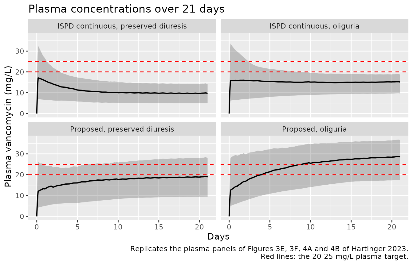
Figures 3E/3F and 4A/4B - peritoneal concentration
The paper plots peritoneal concentrations on a broken axis because the loading dose is two orders of magnitude above the maintenance sawtooth. Day 1 and day 21 are shown separately here for the same reason.
# Replicates the middle "Peritoneal concentrations" panel of Figures 3E/3F/4A/4B.
sim |>
  filter(time <= 24 | time >= 480) |>
  mutate(window = if_else(time <= 24, "Day 1 (loading dose)", "Day 21 (maintenance)"),
         t_in_day = if_else(time <= 24, time, time - 480)) |>
  group_by(treatment, window, t_in_day) |>
  summarise(Q025 = quantile(Cip, 0.025), Q50 = median(Cip),
            Q975 = quantile(Cip, 0.975), .groups = "drop") |>
  ggplot(aes(t_in_day, Q50)) +
  geom_ribbon(aes(ymin = Q025, ymax = Q975), alpha = 0.25) +
  geom_line(linewidth = 0.5) +
  facet_grid(window ~ treatment, scales = "free_y",
             labeller = labeller(treatment = label_wrap_gen(18))) +
  labs(x = "Time within day (h)", y = "Peritoneal vancomycin (mg/L)",
       title = "Peritoneal dialysate concentrations",
       caption = paste("Replicates the peritoneal panels of Figures 3E, 3F, 4A and 4B",
                       "of Hartinger 2023.\nEach sawtooth tooth is one CAPD dwell;",
                       "the vertical drops are the end-of-dwell drain."))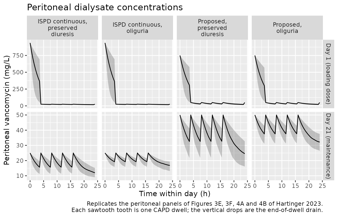
Figures 3E/3F and 4A/4B - AUC24 of peritoneal concentrations
# Replicates the right-hand "AUC of peritoneal concentrations" boxplot panel of
# Figures 3E, 3F, 4A and 4B of Hartinger 2023.
auc_trapz <- function(t, c) sum(diff(t) * (head(c, -1) + tail(c, -1)) / 2)

# Day d spans [24(d-1), 24d] INCLUSIVE at both ends. Assigning days with
# ceiling(time / 24) would push each window's opening record into the previous
# day and drop the highest-concentration half-hour of every dwell cycle, which
# biases AUC24 low by a few percent against the PKNCA interval below.
auc24 <- bind_rows(lapply(auc_days, function(d) {
  sim |>
    filter(time >= 24 * (d - 1), time <= 24 * d, time %in% fine_times) |>
    group_by(treatment, id) |>
    summarise(day = d, auc24 = auc_trapz(time, Cip), n_pts = n(), .groups = "drop")
}))
stopifnot(all(auc24$n_pts == 49L))   # 0-24 h at 0.5 h; a partial window is a bug

auc24 |>
  ggplot(aes(factor(day), auc24)) +
  geom_boxplot(outlier.size = 0.4) +
  geom_hline(yintercept = 400, linetype = "dashed", colour = "red") +
  facet_wrap(~treatment) +
  scale_y_log10() +
  labs(x = "Day", y = "AUC24 of peritoneal concentrations (mg*h/L)",
       title = "Daily peritoneal AUC24",
       caption = paste("Replicates the AUC boxplot panels of Figures 3E, 3F, 4A and 4B of",
                       "Hartinger 2023, on the four days\ncarried at the fine observation",
                       "grid rather than all 21. Red line: the 400 mg*h/L target."))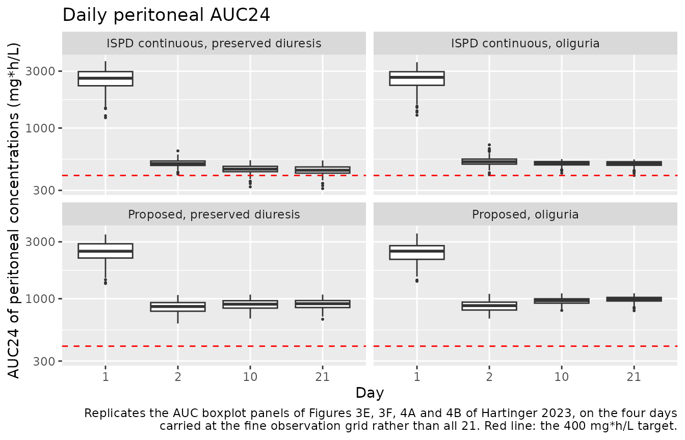
PKNCA validation
NCA is run over the day-21 dwell cycle (480-504 h), i.e. a
steady-state 24-hour CAPD day, separately for the two endpoints. The
peritoneal auclast over that window is exactly the AUC24
the paper’s boxplots report.
nca_window <- c(480, 504)

nca_conc <- sim |>
  filter(!is.na(Cc), time >= nca_window[1], time <= nca_window[2], time %in% fine_times) |>
  select(id, time, treatment, Cc, Cip)

# The exchange starting at 480 h anchors the interval.
nca_dose <- events |>
  filter(evid == 5, time == nca_window[1]) |>
  select(id, time, amt, treatment)

intervals <- data.frame(
  start = nca_window[1], end = nca_window[2],
  auclast = TRUE, cmax = TRUE, cmin = TRUE, tmax = TRUE, cav = TRUE
)

run_nca <- function(conc_col) {
  d <- nca_conc |> mutate(conc = .data[[conc_col]])
  PKNCA::pk.nca(PKNCA::PKNCAdata(
    PKNCA::PKNCAconc(d, conc ~ time | treatment + id),
    PKNCA::PKNCAdose(nca_dose, amt ~ time | treatment + id),
    intervals = intervals
  ))
}

nca_perit  <- run_nca("Cip")
nca_plasma <- run_nca("Cc")

nca_wide <- function(res, tag) {
  as.data.frame(res) |>
    filter(!is.na(PPORRES)) |>
    group_by(treatment, PPTESTCD) |>
    summarise(value = median(PPORRES), .groups = "drop") |>
    mutate(matrix = tag)
}

bind_rows(nca_wide(nca_perit, "Peritoneal dialysate"),
          nca_wide(nca_plasma, "Plasma")) |>
  pivot_wider(names_from = PPTESTCD, values_from = value) |>
  arrange(matrix, treatment) |>
  select(matrix, treatment, cmax, cmin, cav, tmax, auclast) |>
  rename("Matrix" = matrix, "Regimen" = treatment, "Cmax (mg/L)" = cmax,
         "Cmin (mg/L)" = cmin, "Cav (mg/L)" = cav, "Tmax (h)" = tmax,
         "AUC0-24 (mg*h/L)" = auclast) |>
  knitr::kable(digits = 1,
caption = "Median steady-state (day 21) NCA by regimen and matrix.")| Matrix | Regimen | Cmax (mg/L) | Cmin (mg/L) | Cav (mg/L) | Tmax (h) | AUC0-24 (mg*h/L) |
|---|---|---|---|---|---|---|
| Peritoneal dialysate | ISPD continuous, oliguria | 25.0 | 16.8 | 21.0 | 0.0 | 503.0 |
| Peritoneal dialysate | ISPD continuous, preserved diuresis | 25.0 | 12.0 | 18.4 | 0.0 | 442.5 |
| Peritoneal dialysate | Proposed, oliguria | 50.0 | 32.2 | 41.3 | 0.0 | 992.0 |
| Peritoneal dialysate | Proposed, preserved diuresis | 50.0 | 24.5 | 37.9 | 0.0 | 908.5 |
| Plasma | ISPD continuous, oliguria | 15.3 | 15.2 | 15.2 | 18.0 | 365.9 |
| Plasma | ISPD continuous, preserved diuresis | 9.9 | 9.7 | 9.8 | 18.0 | 235.4 |
| Plasma | Proposed, oliguria | 28.7 | 28.4 | 28.6 | 18.5 | 686.4 |
| Plasma | Proposed, preserved diuresis | 19.1 | 18.8 | 19.0 | 18.5 | 456.4 |
Comparison against the published simulations
Hartinger 2023 reports no observed-data NCA table; what it does publish is a set of model-based simulations for exactly the four regimens above, from which median values can be read directly off the figure axes. The reference column below is therefore digitised from the paper’s own figures (Figures 3E, 3F, 4A, 4B - the plasma median trace at day 21 and the day-21 box median of the peritoneal AUC24 panel), not transcribed from a table. Gridline resolution limits the read to roughly the nearest 25 mg*h/L on the AUC axes and the nearest 0.5 mg/L on the plasma axes.
# Digitised from Hartinger 2023 Figures 3E, 3F, 4A, 4B (day-21 values).
published <- tibble::tribble(
  ~treatment,                            ~auclast, ~cav,
  "ISPD continuous, preserved diuresis",      435,  10.0,
  "ISPD continuous, oliguria",                485,  14.2,
  "Proposed, preserved diuresis",             855,  19.0,
  "Proposed, oliguria",                       950,  27.5
)

# `auclast` is the peritoneal AUC24 (the paper's boxplot); `cav` is compared
# against the plasma median trace, which is flat across the day-21 dwell cycle.
sim_for_cmp <- bind_rows(
  as.data.frame(nca_perit)  |> filter(PPTESTCD == "auclast"),
  as.data.frame(nca_plasma) |> filter(PPTESTCD == "cav")
) |>
  mutate(treatment = as.character(treatment))

cmp <- nlmixr2lib::ncaComparisonTable(
  simulated     = sim_for_cmp,
  reference     = published,
  by            = "treatment",
  units         = c(auclast = "mg*h/L", cav = "mg/L"),
  tolerance_pct = 20
)

knitr::kable(
  cmp,
  caption = paste("Simulated day-21 medians vs values digitised from Hartinger 2023",
                  "Figures 3E/3F/4A/4B. auclast = peritoneal AUC24;",
                  "cav = mean plasma concentration. * differs by > 20%."),
  align = c("l", "l", "r", "r", "r")
)| NCA parameter | treatment | Reference | Simulated | % diff |
|---|---|---|---|---|
| AUClast (mg*h/L) | ISPD continuous, preserved diuresis | 435 | 443 | +1.7% |
| AUClast (mg*h/L) | ISPD continuous, oliguria | 485 | 503 | +3.7% |
| AUClast (mg*h/L) | Proposed, preserved diuresis | 855 | 908 | +6.3% |
| AUClast (mg*h/L) | Proposed, oliguria | 950 | 992 | +4.4% |
| Cavg (mg/L) | ISPD continuous, preserved diuresis | 10 | 9.81 | -1.9% |
| Cavg (mg/L) | ISPD continuous, oliguria | 14.2 | 15.2 | +7.4% |
| Cavg (mg/L) | Proposed, preserved diuresis | 19 | 19 | +0.1% |
| Cavg (mg/L) | Proposed, oliguria | 27.5 | 28.6 | +4.0% |
# The percent differences are recomputed here from the raw medians rather than
# parsed back out of the formatted table, and the gate asserts it actually had
# all eight comparisons to test (a lookup that matches nothing passes
# vacuously).
gate <- sim_for_cmp |>
  group_by(treatment, PPTESTCD) |>
  summarise(simulated = median(PPORRES), .groups = "drop") |>
  inner_join(
    published |> pivot_longer(-treatment, names_to = "PPTESTCD",
                              values_to = "reference"),
    by = c("treatment", "PPTESTCD")
  ) |>
  mutate(pct = 100 * (simulated - reference) / reference)

stopifnot(nrow(gate) == 8L, nrow(cmp) == 8L, !anyNA(gate$pct))

# Realised 0.1-7.4% across these eight comparisons. 20 is the package's
# standard tolerance; it sits far enough above that spread to survive a
# different cohort draw, while a mis-transcribed clearance, volume, dose or
# dwell schedule moves these by tens of percent and still breaks the gate.
stopifnot(max(abs(gate$pct)) < 20)
Structural checks
These quantities are deterministic - they depend on the transcribed parameters and the event table alone, not on which cohort was drawn - so they are asserted exactly.
typ <- sim_typ |> group_by(treatment) |> summarise(
  cip_ld   = max(Cip),
  cip_md   = max(Cip[time > 24]),
  vc       = first(vc),
  cl       = first(cl),
  q        = first(q),
  .groups  = "drop"
)

checks <- tibble::tribble(
  ~Claim, ~Source, ~Expected, ~Achieved,
  "Peritoneal peak after a 25 mg/kg loading dose in 2 L = 937.5 mg/L",
  "Fig 3E/3F peritoneal axis (broken axis at ~937)", 937.5,
  typ$cip_ld[typ$treatment == "ISPD continuous, preserved diuresis"],

  "Peritoneal peak after a 20 mg/kg loading dose in 2 L = 750 mg/L",
  "Fig 4A/4B peritoneal axis (broken axis at 750)", 750,
  typ$cip_ld[typ$treatment == "Proposed, preserved diuresis"],

  "Maintenance peritoneal peak, ISPD 25 mg/L in each dwell",
  "Fig 3E/3F peritoneal sawtooth", 25,
  typ$cip_md[typ$treatment == "ISPD continuous, preserved diuresis"],

  "Maintenance peritoneal peak, proposed 50 mg/L in each dwell",
  "Fig 4A/4B peritoneal sawtooth (axis top 50)", 50,
  typ$cip_md[typ$treatment == "Proposed, preserved diuresis"],

  "Typical V2 at BW = 75 kg = 23.6 + 50.9 L",
  "Table 2 equation V2i = V2p + theta_BWV x (BW/75)", 74.5,
  typ$vc[1],

  "Typical CL with oliguria = CLp",
  "Table 2: exponent (RESDIU>500) = 0", 0.192,
  typ$cl[typ$treatment == "ISPD continuous, oliguria"],

  "Typical CL with preserved diuresis at the median eGFR = CLp x 2.26",
  "Table 2: CLp x ((1 + 1.26) x (6.76/6.76))", 0.192 * 2.26,
  typ$cl[typ$treatment == "ISPD continuous, preserved diuresis"],

  "Q = 0.544 L/h",
  "Table 2 row Q", 0.544, typ$q[1]
) |>
  mutate(`Relative error (%)` = 100 * abs(Achieved - Expected) / Expected)

checks |>
  rename("Expected value" = Expected, "Model value" = Achieved) |>
  knitr::kable(digits = c(0, 0, 3, 3, 4),
caption = "Deterministic structural identities.")| Claim | Source | Expected value | Model value | Relative error (%) |
|---|---|---|---|---|
| Peritoneal peak after a 25 mg/kg loading dose in 2 L = 937.5 mg/L | Fig 3E/3F peritoneal axis (broken axis at ~937) | 937.500 | 937.500 | 0 |
| Peritoneal peak after a 20 mg/kg loading dose in 2 L = 750 mg/L | Fig 4A/4B peritoneal axis (broken axis at 750) | 750.000 | 750.000 | 0 |
| Maintenance peritoneal peak, ISPD 25 mg/L in each dwell | Fig 3E/3F peritoneal sawtooth | 25.000 | 25.000 | 0 |
| Maintenance peritoneal peak, proposed 50 mg/L in each dwell | Fig 4A/4B peritoneal sawtooth (axis top 50) | 50.000 | 50.000 | 0 |
| Typical V2 at BW = 75 kg = 23.6 + 50.9 L | Table 2 equation V2i = V2p + theta_BWV x (BW/75) | 74.500 | 74.500 | 0 |
| Typical CL with oliguria = CLp | Table 2: exponent (RESDIU>500) = 0 | 0.192 | 0.192 | 0 |
| Typical CL with preserved diuresis at the median eGFR = CLp x 2.26 | Table 2: CLp x ((1 + 1.26) x (6.76/6.76)) | 0.434 | 0.434 | 0 |
| Q = 0.544 L/h | Table 2 row Q | 0.544 | 0.544 | 0 |
The paper’s qualitative conclusions follow from the same simulation.
med_auc <- auc24 |> filter(day == 21) |> group_by(treatment) |>
  summarise(auc = median(auc24), .groups = "drop")
med_cc <- sim |> filter(time == 504) |> group_by(treatment) |>
  summarise(cc = median(Cc), .groups = "drop")
get <- function(d, col, arm) {
  v <- d[[col]][as.character(d$treatment) == arm]
  if (length(v) != 1L) stop("no unique row for arm '", arm, "'")
  v
}

claims <- tibble::tribble(
  ~Claim, ~Value, ~Pass,
  paste("ISPD continuous dosing is 'borderline efficacious' in patients with",
        "preserved diuresis: peritoneal AUC24 sits just at the 400 mg*h/L target"),
  get(med_auc, "auc", "ISPD continuous, preserved diuresis"),
  abs(get(med_auc, "auc", "ISPD continuous, preserved diuresis") - 400) < 150,

  paste("Oliguric patients on continuous dosing are 'the only subgroup with",
        "relatively reliable intraperitoneal exposure' - higher AUC24 than",
        "the preserved-diuresis arm"),
  get(med_auc, "auc", "ISPD continuous, oliguria"),
  get(med_auc, "auc", "ISPD continuous, oliguria") >
    get(med_auc, "auc", "ISPD continuous, preserved diuresis"),

  paste("On ISPD continuous dosing 'most of the patients would not reach even",
        "the target therapeutic plasmatic level of 20-25 mg/L'"),
  get(med_cc, "cc", "ISPD continuous, preserved diuresis"),
  get(med_cc, "cc", "ISPD continuous, preserved diuresis") < 20,

  paste("The proposed regimen 'yields sufficient exposure in the peritoneum':",
        "peritoneal AUC24 comfortably above 400 mg*h/L"),
  get(med_auc, "auc", "Proposed, preserved diuresis"),
  get(med_auc, "auc", "Proposed, preserved diuresis") > 600,

  paste("In patients with preserved diuresis the proposed regimen raises plasma",
        "towards, but not above, the 20-25 mg/L target - 'without overdosing",
        "patients with excessive plasma levels'"),
  get(med_cc, "cc", "Proposed, preserved diuresis"),
  get(med_cc, "cc", "Proposed, preserved diuresis") > 15 &&
    get(med_cc, "cc", "Proposed, preserved diuresis") < 25,

  paste("The proposed regimen 'may lead to a slight overdose in some",
        "(especially oliguric)' patients - median plasma above 25 mg/L"),
  get(med_cc, "cc", "Proposed, oliguria"),
  get(med_cc, "cc", "Proposed, oliguria") > 25
)

claims |>
  mutate(Value = round(Value, 1)) |>
  rename("Paper claim (Results 3.2 / Discussion)" = Claim,
         "Simulated day-21 median" = Value) |>
knitr::kable(caption = "Hartinger 2023 conclusions reproduced from the packaged model.")| Paper claim (Results 3.2 / Discussion) | Simulated day-21 median | Pass |
|---|---|---|
| ISPD continuous dosing is ‘borderline efficacious’ in patients with preserved diuresis: peritoneal AUC24 sits just at the 400 mg*h/L target | 442.7 | TRUE |
| Oliguric patients on continuous dosing are ‘the only subgroup with relatively reliable intraperitoneal exposure’ - higher AUC24 than the preserved-diuresis arm | 503.0 | TRUE |
| On ISPD continuous dosing ‘most of the patients would not reach even the target therapeutic plasmatic level of 20-25 mg/L’ | 9.7 | TRUE |
| The proposed regimen ‘yields sufficient exposure in the peritoneum’: peritoneal AUC24 comfortably above 400 mg*h/L | 908.7 | TRUE |
| In patients with preserved diuresis the proposed regimen raises plasma towards, but not above, the 20-25 mg/L target - ‘without overdosing patients with excessive plasma levels’ | 18.9 | TRUE |
| The proposed regimen ‘may lead to a slight overdose in some (especially oliguric)’ patients - median plasma above 25 mg/L | 28.6 | TRUE |
The clearance the model gives a patient with preserved diuresis at the median eGFR, 0.434 L/h, is also close to the 0.443 L/h non-dialysis vancomycin clearance the paper’s Discussion cites for high-flux haemodialysis patients - an independent plausibility anchor the paper draws itself.
Assumptions and deviations
Reference values in the comparison table are digitised from the paper’s figures, not read from a table. Hartinger 2023 publishes no NCA table; the only quantitative simulation output it reports is Figures 3 and 4. The four peritoneal AUC24 values and four plasma concentrations in the reference column were read off those axes to roughly the nearest 25 mg*h/L and 0.5 mg/L respectively. The digitisation affects only the comparison table - no parameter value in the model file comes from a figure.
V2pfollows Table 2’s printed equation, not the Results sentence. The Results text says that for a typical 75 kg patientV2is “23.6 L (78%)”, but the printed covariate equationV2i = V2p + theta_BWV x (BW/75)gives 74.5 L at 75 kg. Three things settle it in favour of the equation. The quoted “23.6 L (78%)” is verbatim the Table 2 population row with its RSE, so the sentence is quoting the intercept rather than a typical value. The paper reports that adding this covariate raised theV2pRSE from 9% to 78%, which is the signature of an intercept that no longer carries the typical volume. And the paper’s own Figure 3E/3F show a day-1 plasma concentration near 16 mg/L after a 25 mg/kg intraperitoneal loading dose, which needsV2near 75 L; at 23.6 L it would be roughly 50 mg/L, three times off the published figure. Encoding the equation reproduces all four published panels (see the comparison table); encoding 23.6 L reproduces none.Residual-error values are read as NONMEM
$SIGMAvariances. Table 2 gives 0.091, 4.72 and 0.00604 with no units or percent signs, while every IIV row in the same table is explicitly a percentage; the analysis is NONMEM 7.4.0, whose$SIGMAblock reports variances. They are therefore square-rooted to the SD scale nlmixr2 expects: 30.2% proportional on peritoneal dialysate, 2.17 mg/L additive plus 7.8% proportional on plasma. The alternative reading - that the numbers are already on the SD/CV scale - is rejected because it makes the plasma proportional error 0.6%, which is far below any plausible nephelometric assay imprecision and would make the term pointless alongside a 4.72 mg/L additive component. Nothing in the paper’s figures discriminates the two readings, because the published bands are individual predicted concentrations and so exclude residual error entirely.IIV percentages are converted with the exact log-normal relation
omega^2 = log(1 + CV^2). The paper states the random effects are log-normally distributed but does not say which of the two conventional CV-to-omega formulas it used; the approximationomega = CVwould changeomegaby 3% on CL and 6% on Q.Three occasions are encoded for the inter-occasion variability on
Q. The paper reports one shared IOV magnitude (31% CV) across 57 treatment occasions in 41 patients but never states a maximum occasion count per patient. Occasions 2 and 3 arefix()’d to the occasion-1 variance to reproduce NONMEM’s$OMEGA BLOCK(1) SAME. A single-episode simulation such as this one usesOCC = 1throughout, so the IOV contributes one extra draw onQper subject - which is exactly its role in the paper’s own simulations.eGFR is undefined in oliguric subjects. Table 1 states eGFR was computed “only in patients with preserved diuresis”. Because the preserved-diuresis indicator is the exponent on the whole bracket, the eGFR ratio is raised to the power 0 in oliguric subjects and drops out; the cohort above supplies the median 6.76 as a placeholder, which changes nothing.
The peritoneal cavity is declared a paper-specific compartment. There is no canonical
peritoneumininst/references/compartment-names.md. It is declared throughpaper_specific_compartments, matchingRoyer_2011_cisplatin.R, which carries the same anatomical state for intraperitoneal perioperative chemotherapy. Hartinger 2023 is the second independent paper in the library to need it, which is the trigger to consider promoting the name to canonical; that is a register decision left to review.Drainage is assumed complete at the end of each dwell. The paper’s Figure 1 distinguishes
VOL INfromVOL OUTbut Table 2 fixes onlyV1, to the instilled volume, and reports no residual-volume or ultrafiltration parameter. The complete-drain reading is what the published figures show: a maintenance dose of 25 or 50 mg/L peaks at exactly 25 or 50 mg/L in every dwell, with no dwell-to-dwell carry-over, and both loading-dose peaks land exactly ondose / 2 L.The assay correction is upstream of the model. Glucose-based dialysate depressed the nephelometric vancomycin measurement by about 20%, and all peritoneal concentrations were multiplied by 1.2885 before modelling (Methods 2.2, Figure S1).
Cipis therefore on the corrected scale; raw assay values from a glucose-based solution must be corrected before they are compared with it.