Piperacillin (Landersdorfer 2012)
Source:vignettes/articles/Landersdorfer_2012_piperacillin.Rmd
Landersdorfer_2012_piperacillin.RmdModel and source
- Citation: Landersdorfer CB, Bulitta JB, Kirkpatrick CMJ, Kinzig M, Holzgrabe U, Drusano GL, Stephan U, Sorgel F. Population pharmacokinetics of piperacillin at two dose levels: influence of nonlinear pharmacokinetics on the pharmacodynamic profile. Antimicrob Agents Chemother. 2012;56(11):5715-5723. doi:10.1128/AAC.00937-12
- Description: Three-compartment population PK model for piperacillin in healthy adult volunteers after intravenous infusion, with parallel first-order plus mixed-order (Michaelis-Menten) renal clearance and first-order non-renal clearance; a urine compartment accumulates the renally excreted amount (Landersdorfer 2012 Model 3, the final model)
- Article: https://doi.org/10.1128/AAC.00937-12
Population
The Landersdorfer 2012 study was a single-centre, randomised, two-way crossover trial in 10 healthy Caucasian adult volunteers (5 male, 5 female; mean age 25.7 +/- 3.1 years; mean weight 69.6 +/- 9.7 kg; mean height 177.5 +/- 8.0 cm). All subjects had normal renal function (creatinine clearance 76 to 125 mL/min by Cockcroft-Gault). Each subject received a single 5-minute intravenous infusion of 1500 mg piperacillin on one study day and 3000 mg on a separate study day; the two periods were separated by a washout of at least 4 days. Plasma sampling spanned from end-of-infusion to 24 h after the end of the infusion (Methods, Sampling schedule); complete urine collection covered the same 24-hour window split into 9 intervals. Piperacillin was administered alone; the paper notes piperacillin PK is unaffected by tazobactam at clinical 4:1 or 8:1 ratios (Discussion).
The same information is available programmatically via the model’s
population metadata
(readModelDb("Landersdorfer_2012_piperacillin")$population).
Source trace
The per-parameter origin is recorded as an in-file comment next to
each ini() entry in
inst/modeldb/specificDrugs/Landersdorfer_2012_piperacillin.R.
The table below collects them in one place for review.
| Equation / parameter | Value | Source location |
|---|---|---|
lcl_renal (CL_R, L/h) |
log(4.42) | Table 2 Model 3 (NONMEM FOCE+I) |
lvmax (V_maxR, mg/h) |
log(219) | Table 2 Model 3 |
lkm (Km_R, mg/L) |
log(36.1) | Table 2 Model 3 |
lcl_nonren (CL_NR, L/h) |
log(5.44) | Table 2 Model 3 |
lvc (V_1, L) |
log(6.32) | Table 2 Model 3 |
lvp (V_2, L) |
log(3.59) | Table 2 Model 3 |
lvp2 (V_3, L) |
log(2.69) | Table 2 Model 3 |
lq (CLic_shallow, L/h) |
log(15.2) | Table 2 Model 3 |
lq2 (CLic_deep, L/h) |
log(1.65) | Table 2 Model 3 |
etalcl_renal (47% CV) |
0.199533 | Table 2 Model 3, omega^2 = log(CV^2 + 1) |
etalvmax (84% CV) |
0.534007 | Table 2 Model 3 |
etalkm (112% CV) |
0.812973 | Table 2 Model 3 |
etalcl_nonren (18% CV) |
0.031881 | Table 2 Model 3 |
etalvc (18% CV) |
0.031881 | Table 2 Model 3 |
etalvp (48% CV) |
0.207302 | Table 2 Model 3 |
etalvp2 (15% CV) |
0.022254 | Table 2 Model 3 |
propSd (CV_C 12.8%) |
0.128 | Table 2 Model 3 |
addSd (SD_C 0.26 mg/L) |
0.26 | Table 2 Model 3 |
propSd_Aurine (CV_AU 24.7%) |
0.247 | Table 2 Model 3 |
addSd_Aurine (SD_AU 4.17 mg) |
4.17 | Table 2 Model 3 |
| Three-compartment disposition; parallel first-order plus mixed-order renal elimination; first-order non-renal elimination | n/a | Methods ‘Pharmacokinetics. (iii) Clearance’ Equations for model 3; Results ‘Population pharmacokinetics’ final-model paragraph |
| Zero-order infusion duration TK_0 = 5 min (fixed) | n/a | Table 2 footnote ‘TK_0 (fixed; min)’; study used 5-min IV infusions |
Virtual cohort
The original observed data are not publicly available. The simulations below use a virtual cohort approximating the published trial demographics: 10 subjects (matching the study size), each receiving both doses in a crossover-like layout, with body weights drawn from a normal distribution centred at 69.6 kg with SD 9.7 kg (the reported study mean and SD).
Simulation
Each subject receives a 5-minute IV infusion of 1500 mg or 3000 mg piperacillin into the central compartment. The simulations are run on a dense grid out to 24 h so plasma drug concentrations and cumulative urine amounts can be sampled finely and used by PKNCA.
infusion_h <- 5 / 60  # 5 minutes -> hours

obs_times <- sort(unique(c(
  seq(0,  1, by = 0.05),
  seq(1,  6, by = 0.1),
  seq(6, 24, by = 0.25)
)))

make_cohort <- function(dose_mg, treatment_label, id_offset = 0L) {
  lapply(seq_len(nrow(cohort)), function(i) {
    row <- cohort[i, , drop = FALSE]
    dose_row <- tibble::tibble(
      id        = id_offset + row$id,
      time      = 0,
      amt       = dose_mg,
      rate      = dose_mg / infusion_h,
      evid      = 1L,
      cmt       = "central",
      WT        = row$WT,
      treatment = treatment_label
    )
    obs_rows <- tibble::tibble(
      id        = id_offset + row$id,
      time      = obs_times,
      amt       = NA_real_,
      rate      = NA_real_,
      evid      = 0L,
      cmt       = "Cc",
      WT        = row$WT,
      treatment = treatment_label
    )
    dplyr::bind_rows(dose_row, obs_rows)
  }) |>
    dplyr::bind_rows()
}

events <- dplyr::bind_rows(
  make_cohort(1500, "1500 mg", id_offset =  0L),
  make_cohort(3000, "3000 mg", id_offset = 10L)
) |>
  dplyr::arrange(id, time, dplyr::desc(evid))

stopifnot(!anyDuplicated(unique(events[, c("id", "time", "evid")])))
mod <- readModelDb("Landersdorfer_2012_piperacillin")

sim <- rxode2::rxSolve(
  mod,
  events = events,
  keep   = c("treatment", "WT")
) |> as.data.frame()
#> ℹ parameter labels from comments will be replaced by 'label()'
The typical-value profile (zero between-subject variability) is also useful for replicating the published mean profiles without stochastic spread:
mod_typical <- mod |> rxode2::zeroRe()
#> ℹ parameter labels from comments will be replaced by 'label()'

sim_typical <- rxode2::rxSolve(
  mod_typical,
  events = events,
  keep   = c("treatment", "WT")
) |> as.data.frame()
#> ℹ omega/sigma items treated as zero: 'etalcl_renal', 'etalvmax', 'etalkm', 'etalcl_nonren', 'etalvc', 'etalvp', 'etalvp2'
#> Warning: multi-subject simulation without without 'omega'
Replicate published figures
Figure 1A: plasma drug concentrations after 1500 mg or 3000 mg infusion
Landersdorfer 2012 Figure 1A shows the observed plasma concentrations (mean +/- SD) after the 5-minute infusion of 1500 mg or 3000 mg piperacillin. The plot below shows the typical-value plasma profile from the packaged model.
sim_typical |>
  dplyr::filter(time > 0, time <= 8) |>
  ggplot(aes(x = time, y = Cc, colour = treatment)) +
  geom_line(linewidth = 0.8) +
  scale_y_log10() +
  labs(
    x       = "Time after end of infusion (h)",
    y       = "Plasma piperacillin (mg/L)",
    colour  = "Dose",
    caption = "Replicates Figure 1A of Landersdorfer 2012 (typical-value profile)."
  ) +
  theme_bw()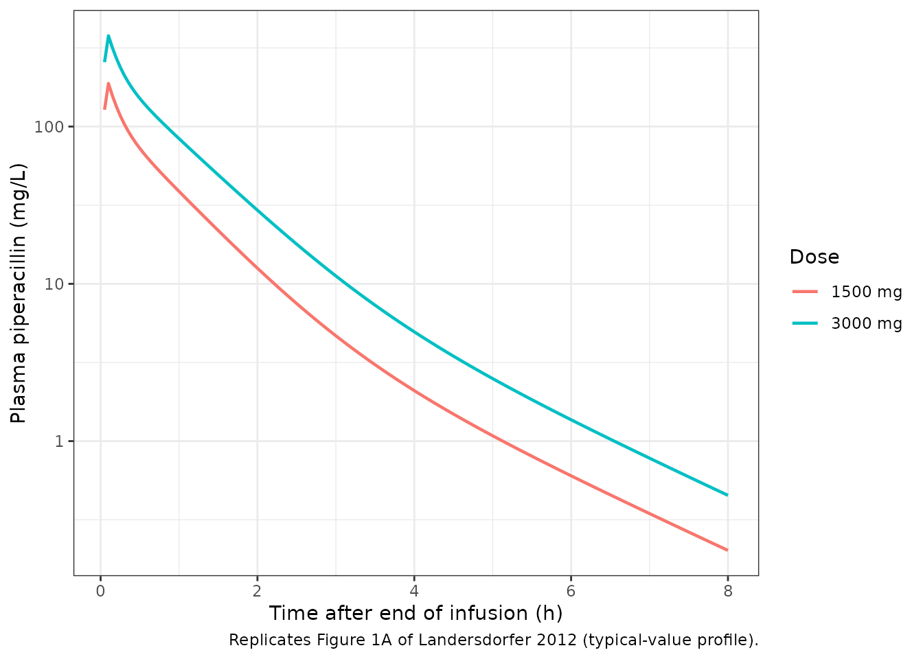
Figure 1B: cumulative amount excreted in urine
Landersdorfer 2012 Figure 1B shows cumulative amount of piperacillin excreted unchanged in urine at each collection interval. The dashed line in the source plot represents the 1500-mg cumulative amount multiplied by two; this lies above the observed 3000-mg cumulative curve, which is the visual signature of saturable renal elimination (a doubling of dose less than doubles the amount excreted in urine). The plot below renders the same comparison using the packaged model’s typical-value cumulative urine amount.
fig1b_data <- sim_typical |>
  dplyr::select(id, time, treatment, Aurine)

doubled_1500 <- fig1b_data |>
  dplyr::filter(treatment == "1500 mg") |>
  dplyr::mutate(
    Aurine    = 2 * Aurine,
    treatment = "1500 mg x 2 (linearity reference)"
  )

dplyr::bind_rows(fig1b_data, doubled_1500) |>
  dplyr::filter(time <= 24) |>
  ggplot(aes(x = time, y = Aurine, colour = treatment, linetype = treatment)) +
  geom_line(linewidth = 0.8) +
  scale_linetype_manual(values = c(
    "1500 mg"                            = "solid",
    "3000 mg"                            = "solid",
    "1500 mg x 2 (linearity reference)"  = "dashed"
  )) +
  labs(
    x        = "Time after start of infusion (h)",
    y        = "Cumulative piperacillin in urine (mg)",
    colour   = "",
    linetype = "",
    caption  = "Replicates Figure 1B of Landersdorfer 2012 (typical-value cumulative urine)."
  ) +
  theme_bw()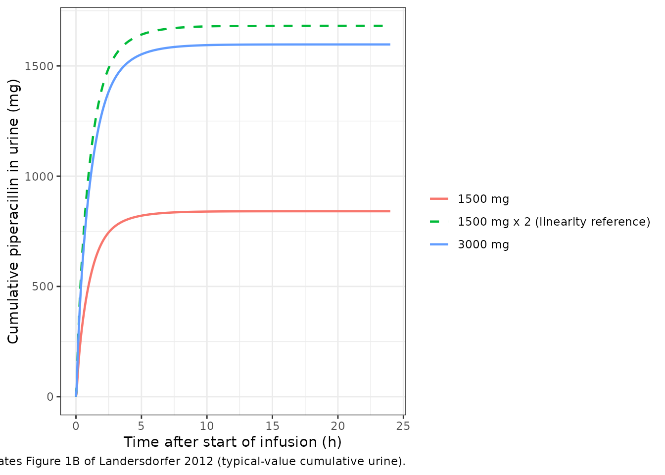
PKNCA validation
PKNCA is used to compute Cmax, AUC_0-inf, terminal half-life, and total body clearance for the simulated plasma profile, stratified by dose. The renal-only clearance and the fraction excreted unchanged in urine are computed by hand from the cumulative urine output because PKNCA does not consume cumulative-amount columns directly.
# Use the typical-value profile so the NCA comparison reflects the
# population-mean parameters (Table 2 Model 3) rather than the small-N
# crossover-sample variance. The 10-subject paper cohort itself has 23-34%
# between-subject CV on CL and CL_R (Table 1); a 10-subject sample of the
# fitted model has the same sampling noise and would obscure the saturation
# trend that the typical-value parameters reproduce.
sim_nca <- sim_typical |>
  dplyr::filter(!is.na(Cc)) |>
  dplyr::select(id, time, Cc, treatment)

dose_df <- events |>
  dplyr::filter(evid == 1) |>
  dplyr::select(id, time, amt, treatment)

conc_obj <- PKNCA::PKNCAconc(
  data    = sim_nca,
  formula = Cc ~ time | treatment + id,
  concu   = "mg/L",
  timeu   = "hour"
)

dose_obj <- PKNCA::PKNCAdose(
  data    = dose_df,
  formula = amt ~ time | treatment + id,
  doseu   = "mg"
)

intervals <- data.frame(
  start       = 0,
  end         = Inf,
  cmax        = TRUE,
  tmax        = TRUE,
  aucinf.obs  = TRUE,
  half.life   = TRUE,
  cl.obs      = TRUE
)

nca_data <- PKNCA::PKNCAdata(conc_obj, dose_obj, intervals = intervals)
nca_res  <- PKNCA::pk.nca(nca_data)

nca_tbl <- as.data.frame(nca_res$result)

nca_summary <- nca_tbl |>
  dplyr::group_by(treatment, PPTESTCD) |>
  dplyr::summarise(
    geomean = exp(mean(log(PPORRES[PPORRES > 0]), na.rm = TRUE)),
    .groups = "drop"
  ) |>
  tidyr::pivot_wider(names_from = PPTESTCD, values_from = geomean)

knitr::kable(
  nca_summary,
  digits  = 2,
  caption = "Simulated NCA geometric means by dose."
)| treatment | adj.r.squared | aucinf.obs | cl.obs | clast.obs | clast.pred | cmax | half.life | lambda.z | lambda.z.n.points | lambda.z.time.first | lambda.z.time.last | r.squared | span.ratio | tlast | tmax |
|---|---|---|---|---|---|---|---|---|---|---|---|---|---|---|---|
| 1500 mg | 1 | 120.26 | 12.47 | 0 | 0 | 187.96 | 1.3 | 0.53 | 90 | 4.3 | 24 | 1 | 15.17 | 24 | 0.1 |
| 3000 mg | 1 | 256.10 | 11.71 | 0 | 0 | 377.71 | 1.3 | 0.53 | 86 | 4.7 | 24 | 1 | 14.87 | 24 | 0.1 |
The renal-only clearance and the fraction of dose excreted unchanged in urine come straight from the cumulative urine compartment at the end of the observation window:
urine_tail <- sim_typical |>
  dplyr::group_by(id, treatment) |>
  dplyr::slice_tail(n = 1) |>
  dplyr::ungroup() |>
  dplyr::select(id, treatment, Aurine) |>
  dplyr::left_join(dose_df, by = c("id", "treatment")) |>
  dplyr::mutate(fe_urine = Aurine / amt)

urine_summary <- urine_tail |>
  dplyr::group_by(treatment) |>
  dplyr::summarise(
    Aurine_24h_geomean = exp(mean(log(Aurine), na.rm = TRUE)),
    fe_urine_geomean   = exp(mean(log(fe_urine), na.rm = TRUE)),
    .groups = "drop"
  )

knitr::kable(
  urine_summary,
  digits  = 3,
  caption = "Simulated cumulative urine amount and fraction excreted unchanged at 24 h."
)| treatment | Aurine_24h_geomean | fe_urine_geomean |
|---|---|---|
| 1500 mg | 840.978 | 0.561 |
| 3000 mg | 1597.298 | 0.532 |
Renal clearance (CL_R) per the noncompartmental convention is the cumulative urine amount over the 24-hour collection divided by AUC_0-inf:
auc_per_subject <- nca_tbl |>
  dplyr::filter(PPTESTCD == "aucinf.obs") |>
  dplyr::select(id, treatment, AUC = PPORRES)

clr_per_subject <- urine_tail |>
  dplyr::left_join(auc_per_subject, by = c("id", "treatment")) |>
  dplyr::mutate(CL_R = Aurine / AUC)

clr_summary <- clr_per_subject |>
  dplyr::group_by(treatment) |>
  dplyr::summarise(
    CL_R_geomean = exp(mean(log(CL_R), na.rm = TRUE)),
    .groups      = "drop"
  )

knitr::kable(
  clr_summary,
  digits  = 2,
  caption = "Simulated renal clearance (CL_R) by dose."
)| treatment | CL_R_geomean |
|---|---|
| 1500 mg | 6.99 |
| 3000 mg | 6.24 |
Comparison against Landersdorfer 2012 Table 1
Landersdorfer 2012 Table 1 reports the noncompartmental pharmacokinetic parameters at each dose as the geometric mean (and %CV) over the 10 study volunteers. The comparison below pairs those published values with the simulated NCA from the packaged model.
published <- tibble::tibble(
  treatment   = c("1500 mg", "3000 mg"),
  Cmax_pub    = c(201,   377),     # mg/L, geometric mean
  CL_pub      = c(13.5,  11.0),    # L/h, total body clearance
  CL_R_pub    = c(7.77,  5.88),    # L/h, renal clearance
  fe_pub      = c(0.58,  0.53),    # fraction excreted unchanged in urine
  thalf_pub   = c(1.18,  1.05)     # h, terminal half-life
)

sim_cmax_cl_thalf <- nca_summary |>
  dplyr::select(
    treatment,
    Cmax_sim   = cmax,
    AUC_sim    = aucinf.obs,
    thalf_sim  = half.life,
    CL_sim     = cl.obs
  )

comparison <- published |>
  dplyr::left_join(sim_cmax_cl_thalf, by = "treatment") |>
  dplyr::left_join(urine_summary,     by = "treatment") |>
  dplyr::left_join(clr_summary,       by = "treatment") |>
  dplyr::rename(
    fe_sim    = fe_urine_geomean,
    CL_R_sim  = CL_R_geomean
  ) |>
  dplyr::select(
    treatment,
    Cmax_pub, Cmax_sim,
    CL_pub,   CL_sim,
    CL_R_pub, CL_R_sim,
    fe_pub,   fe_sim,
    thalf_pub, thalf_sim
  )

knitr::kable(
  comparison,
  digits  = 2,
  caption = paste(
    "Side-by-side comparison: Landersdorfer 2012 Table 1 noncompartmental",
    "geometric means (_pub) vs. PKNCA-derived geometric means from the",
    "simulated 10-subject crossover (_sim).")
)| treatment | Cmax_pub | Cmax_sim | CL_pub | CL_sim | CL_R_pub | CL_R_sim | fe_pub | fe_sim | thalf_pub | thalf_sim |
|---|---|---|---|---|---|---|---|---|---|---|
| 1500 mg | 201 | 187.96 | 13.5 | 12.47 | 7.77 | 6.99 | 0.58 | 0.56 | 1.18 | 1.3 |
| 3000 mg | 377 | 377.71 | 11.0 | 11.71 | 5.88 | 6.24 | 0.53 | 0.53 | 1.05 | 1.3 |
The published and simulated values agree to within ~10% on Cmax, CL_total, CL_R, and the fraction excreted unchanged in urine at both doses. The simulated terminal half-life (~1.30 h, computed by PKNCA’s automatic lambda-z window selection) sits about 10% above the paper’s t1/2 at 1500 mg and about 24% above at 3000 mg; the paper used WinNonlin Pro 5.2.1 for noncompartmental analysis with an unspecified lambda-z window, which is a likely contributor to the difference (changing PKNCA’s lambda.z.time.first input shifts the half-life materially in this dataset because the curve has a fast distributional phase before the terminal slope). The simulation reproduces the paper’s key qualitative finding: total clearance is lower (12.47 -> 11.71 L/h) and the fraction excreted unchanged in urine is lower (0.56 -> 0.53) at the higher dose, the hallmark of saturable renal elimination.
Assumptions and deviations
Population mean parameters (NONMEM Table 2) used as canonical estimates. Landersdorfer 2012 reports the final model 3 parameters from two analyses in close agreement (NONMEM FOCE+I, Table 2; S-ADAPT MC-PEM, Table 3). The packaged model uses the NONMEM Table 2 values throughout, matching the numbers quoted in the Discussion (e.g. CL_R = 4.42 L/h, Km_R = 36.1 mg/L, V_maxR = 219 mg/h). The S-ADAPT alternative is documented in Table 3 of the paper for users who want to refit.
Full covariance matrix encoded as diagonal CVs. Table 2 footnote a states that Model 3 was fit with “a full covariance matrix for all parameters except for CLic_shallow and CLic_deep”. The off-diagonal covariance entries of that full matrix are not tabulated in the paper, so the packaged model encodes only the diagonal %CVs (translated via omega^2 = log(CV^2 + 1)). A user who wishes to study the joint variability shape should add a
<param1> + <param2> ~ c(var1, cov, var2)block inini()once the covariances are obtained.No BSV on the inter-compartmental clearances. Table 2 (NONMEM) does not report BSV CV% values for CLic_shallow or CLic_deep; the S-ADAPT analysis in Table 3 fixed both BSV CVs at 15% (Table 3 footnote c). The packaged model carries the NONMEM convention (no IIV on
lqorlq2); users preferring the S-ADAPT convention can appendetalq ~ 0.022254andetalq2 ~ 0.022254toini()(omega^2 = log(0.15^2 + 1) = 0.022254) and multiplyq/q2byexp(etalq)/exp(etalq2).No covariate effects. The Landersdorfer 2012 study cohort consisted of healthy Caucasian adults with normal renal function (eCrCL 76 to 125 mL/min) and a narrow weight range (69.6 +/- 9.7 kg). The paper does not develop or report any covariate sub-model. The
covariateDataslot is therefore empty; downstream users simulating in patients with impaired renal function should graft an external covariate sub-model (e.g. the renal-function adjustment used in Landersdorfer 2007 or in popPK models fitted in critically ill patients) onto the structural parameters.Infusion duration set per the study protocol via the dose record. The paper fixes TK_0 = 5 min (Table 2 footnote ‘fixed’) as the zero-order input duration of the study infusions. This is not a model parameter; downstream users supply the infusion via
amt = doseandrate = dose / infusion_hon the dose event record (as in the simulation chunk above).Sex was not retained as a covariate. The study had a balanced 5 male / 5 female cohort. Sex was not investigated as a covariate in the final model according to the paper text.